Week 5 - Curve fitting

Objective

Write code to fit a linear and cubic polynomial for the Cp data

Introduction

Curve Fitting

Curve fitting is the process of constructing a curve or mathematical function, that has the best fit to a series of data points, possibly subject to constraints. Curve fitting can involve either interpolation, where an exact fit to the data is required, or smoothing, in which a smooth function is constructed that approximately fits the data. A related topic is regression analysis, which focuses more on questions of statistical interference such as how much uncertainty is present in a curve that is fit to data observed with random errors. Fitted curves can be used as an aid for data visualization, to infer values of a function where no data are available, and to summarize the relationships among two or more variables.

Curve fitting can also be described as the process of constructing a curve, or mathematical functions, which possess the closest proximity to the real series of data. By curve fitting, we can mathematically construct the functional relationship between the observed dataset and parameter values, etc.

Solution Procedure

1. We need to import the math library, plot library, and Numpy library for certain calculations and processes. To solve the curve-fitting problem we are going to import curve_fit from the scipy.optimize.

2. Now we are going to define the function for linear polynomial.

y = a*t + b

3. Now we are going to read the data from the 'data' file. We are going to read the data file and then we will separate the temperature and `C_p` data.

4. Now we are going to calculate the coefficient a and b ......................

5. Now we have the formula for the data and we created the curve fit for the data. So now we have to check that the curve fit which we have obtained is good or not. So in order to check that we have to calculate the `R^2` value which is nothing but the quantity that measures that how successful the fit is. In order to calculate that we are going to take the following steps:-

First, we have to calculate the difference between actual `C_p` and predicted `C_p` which is the error.

Now we have to calculate the sum of the square of error(SSE).

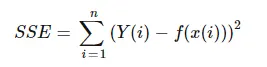
Now we have to calculate the mean of actual specific heat.

Now we have to calculate the sum of the square of regression(SSR).

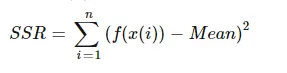
Now we are going to add SSE and SSR values.

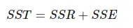
Now we can calculate the `R^2` value. which is the ratio of SSR and SST.

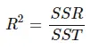
I have calculated the root mean square error (RMSE) also.

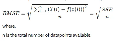
6. The value of `R^2` tells us the curve fit is good or not. If the value is greater than 0.95 then it is a good fit otherwise it is not good. So we want to display it when we execute the program. In order to do that we are going to use the 'if else' command. It checks the value and displays accordingly.

7. Now we are going to compare the curve fit with the original data. In order to do that we are going to plot them in the graph with the 'plot' command.

8. We are going to give the label to the x and y-axis of the plot and we are going to give the title to the figure and we are going to give the legends to the plot.

9. Now we are going to repeat the same steps in order to create the curve fit for the cubic polynomial.

First, we are going to define the function for cubic polynomial.

`y = a*t^3+b*t^2+c*t+d`

So same as before we are going to calculate the coefficient a, b, c, and d. Then we are going to calculate the `C_p`.

After calculating the `C_p` value we are going to check that the curve we have obtained is fit or not with the help of the calculation of the `R^2` value and plot the graph.

Python Script

# Curve Fitting

import math
import matplotlib.pyplot as plt 
import numpy as np 
from scipy.optimize import curve_fit

# Curve Fit Functions

# Linear Function
def  linear(t,a,b):
	return a*t + b


# Reading Data
def read_data():
	temperature = []
	cp = []
	for line in open('data','r'):
		values = line.split(',')
		temperature.append(float(values[0]))
		cp.append(float(values[1]))

	return [temperature,cp]

# main program Linear Fitting
temperature, cp = read_data()
popt, pcov  = curve_fit(linear,temperature,cp)
linear_cp = linear(np.array(temperature), *popt)

#Error
E = abs(cp - linear_cp)

# Number of variable
n = 3200

# Sum of squared error
SSE1 = 0
for i in E:
	
	SSE1 = SSE1 + pow(i,2)

# Mean value calculation
mean_cp = np.mean(cp)

#Sum of squares of the regression
SSR1 = 0
for i in cp:
	SSR1 = SSR1 +  pow((i-mean_cp),2)

# SST is sum of SSE & SSR
SST1 = SSR1 + SSE1

# Root mean squared error
RMSE1 = pow((SSE1/n),0.5)

# Sucess of the fit
R_square1 = SSR1/SST1
print(R_square1)

if R_square1 >= 0.95:
    print('linear polynomial for cp data curve fit is good')
else:
    print('linear polynomial for cp data curve fit is not good')


plt.plot(temperature,cp,color="red",linewidth=3)
plt.plot(temperature,linear_cp,color="blue",linewidth=3)
plt.legend(['Actual Data','Linear Curve Data'])
plt.xlabel('Temperature (K)')
plt.ylabel('Cp')
plt.title('Actual Curve vs Linear Fit Curve')
plt.show()

# Cubic Polynomial Function
def cubic(t,a,b,c,d):
	return a*pow(t,3) + b*pow(t,2) + c*t + d

# main program Cubic Fitting
temperature, cp = read_data()
popt, pcov  = curve_fit(cubic,temperature,cp)
cubic_cp = cubic(np.array(temperature), *popt)

#Error
E1 = abs(cp - cubic_cp)

# Number of variable
n = 3200

# Sum of squared error
SSE2 = 0
for i in E1:
	
	SSE2 = SSE2 + pow(i,2)

# Mean value calculation
mean_cp = np.mean(cp)

#Sum of squares of the regression
SSR2 = 0
for i in cp:
	SSR2 = SSR2 +  pow((i-mean_cp),2)

# SST is sum of SSE & SSR
SST2 = SSR2 + SSE2

# Root mean squared error
RMSE2 = pow((SSE2/n),0.5)

# Sucess of the fit
R_square2 = SSR2/SST2
print(R_square2)

if R_square2 >= 0.95:
    print('Cubic polynomial for cp data curve fit is good')
else:
    print('Cubic polynomial for cp data curve fit is not good')

plt.plot(temperature,cp,color="red",linewidth=3)
plt.plot(temperature,cubic_cp,color="blue",linewidth=3)
plt.legend(['Actual Data','Cubic Curve Data'])
plt.xlabel('Temperature (K)')
plt.ylabel('Cp')
plt.title('Actual Curve vs Cubic Fit Curve')
plt.show()

Output

Now when we execute the program it gives us `R^2` values for both linear and cubic polynomial and tells us that curve fit is good or not.

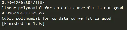
In this program, I have got the value of `R^2` for linear polynomial is 0.9301. Which is less than 0.95 so it displays 'linear polynomial for cp data curve fit is not good'.

And the value of `R^2` for cubic polynomial is 0.9967. Which is greater than 0.95 so it displays 'linear polynomial for cp data curve fit is good'.

Linear fit curve

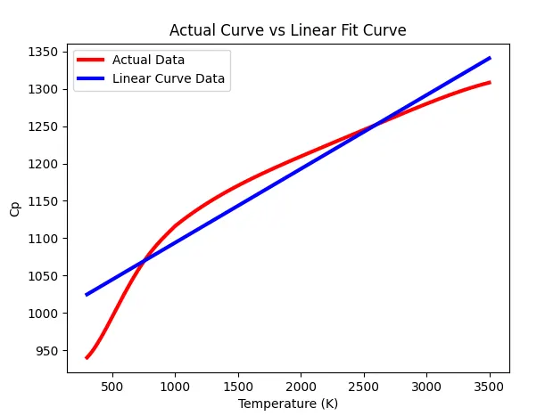
In this curve, we can see the red color curve is the actual `C_p` data curve and the blue color curve represent the curve fit for linear polynomial.

Cubic fit curve

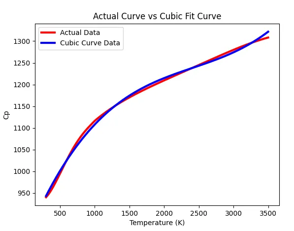
In this curve, we can see the red color curve is the actual `C_p` data curve and the blue color curve represent the curve fit for cubic polynomial.

What does popt and pcov mean?

popt - is a one-dimensional array consisting of optimum values of the coefficients for the polynomial model chosen, each entry matches the order in the function definition.

pcov - is the covariance matrix showing the uncertainty and interdependence of each parameter in popt. The pcov variable contains the covariance matrix, which indicates the uncertainties and correlations between parameters. This is most useful when the data has uncertainties

What does np.array(temperature) do?

It generates an array and stores the different values of the temperature and passes the generated value to the numpy for numerical calculation in python.

What does the * in *popt mean?

It refers to the value in the array popt

What needs to be done in order to make the curve fit perfect?

We can make a curve fit perfect by interpolation. Interpolation is a method of estimating values between known data points. Use interpolation to smooth observed data, fill in missing data, and make predictions.

We can make a curve fit perfect by regression. Regression is a method of estimating the relationship between a response (output) variable and one or more predictor (input) variables. If the output depends on a lesser variable it gives us the more perfect fit.

So to make a perfect fit the difference between the actual measured value and predicted value should be minimum.

Cubic fit can be improved by the Splitwise method.