Week 11 - Simulation of Flow through a pipe in OpenFoam
Objective
Write a program in Matlab that can generate the computational mesh automatically for any wedge angle and grading schemes.
We have to make sure that the number of cells along the "axi symmetric"
We have to show that the velocity profile matches with the Hagen poiseuille's equation
We have to show that the velocity profile is fully developed
And have to show post-process velocity and shear stress
Introduction
We have assumed that the flow is laminar- incompressible-viscous-transient flow through the pipe. Because of this flow of nature, we are going to choose icoFoam solver. We have assumed that fluid is water and the temperature of the water is 20 degrees Celcius.
The fluid is laminar so we are going to take the Reynold number to be 2000. (The Reynolds number, referred to as Re, is used to determine whether the fluid flow is laminar or turbulent.)

The velocity of the fluid in pipe changes from zero at the surface (no slip condition) to maximum at the pipe center and again decreases and goes to the zero at the surface.
The shear stress is maximum at the surface of the pipe and decreases and goes to minimum at the center of the pipe and again increases.
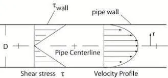
These values are after we got the fully developed velocity profile and shear stress profile.
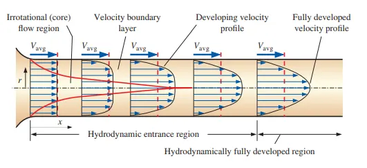
Hydrodynamic entry length
The hydrodynamic entry length is usually taken to be the distance from the pipe entrance to where the wall shear stress (and thus the friction factor) reaches within about 2 percent of the fully developed value. In laminar flow, the nondimensional hydrodynamic entry length is given approximately as
`L_h = 0.05*Re*D`
Hagen poiseuille's equation
Hagen–Poiseuille equation, also known as the Hagen–Poiseuille law, Poiseuille law or Poiseuille equation. This is a physical law that gives the pressure drop in an incompressible and Newtonian fluid in laminar flow flowing through a long cylindrical pipe of the constant cross-section.
Poiseuille's Equation describes the pressure drop due to the viscosity of the fluid.
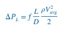
where
`triangleP_L`= pressure drop
`f`= Darcy friction factor = `64/(Re)`(Re = Reynold number)
L = length of the pipe at which we are calculating pressure drop
D = diameter of the pipe
`rho` = density of the fluid
`V_(avg)`= average velocity of the fluid
Wedge Boundary
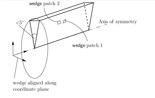
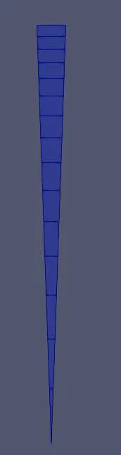
For 2 dimensional axi-symmetric cases, e.g. a cylinder, the geometry is specified as a wedge of small angle (e.g. ) and 1 cell thick running along the plane of symmetry, straddling one of the coordinate planes, as shown in Figure. The axi-symmetric wedge planes must be specified as separate patches of wedge type.
Matlab Script
1. Matlab code to create the blockMeshDict file:-
clear all
close all
clc

% inputs
% angle
theta = 4;
% diameter (m)
D = 0.02;
% radius
R = D/2;
% Reynold number
Re = 2000;
% kinematic viscocity
Nu = 1e-6;


% Hydrodynamic entrance length
L1 = .05*D*Re;
%length of the pipe
L = L1+0.5;

% vertices co-ordinates

% point 0
x0 = 0;
y0 = 0;
z0 = 0;

% point 1
x1 = -R*sind(theta/2);
y1 = R*cosd(theta/2);
z1 = 0;

% point 2
x2 = R*sind(theta/2);
y2 = R*cosd(theta/2);
z2 = 0;

% point 3
x3 = 0;
y3 = 0;
z3 = L;

% point 4
x4 = -R*sind(theta/2);
y4 = R*cosd(theta/2);
z4 = L;

% point 5
x5 = R*sind(theta/2);
y5 = R*cosd(theta/2);
z5 = L;

%point at arc 1-2
x6 = 0;
y6 = R;
z6 = 0;

% point at arc 4-5
x7 = 0;
y7 = R;
z7 = L;

% cells in local axis
nx = 15;
ny = 1;
nz = 500;

% grading factor
gx = 0.2;
gy = 1;
gz = 1;

f1 = fopen('blockMeshDict.txt','w');

fprintf(f1, '/*------------------------*- C++ -*-------------------------*\\\n');
fprintf(f1, '=========                |\n');
fprintf(f1, '\\\\      / F ield         | OpenFOAM:  The Source CFD Toolbox\n');
fprintf(f1, ' \\\\    /  O peration     | Website:   https://openfoam.org\n');
fprintf(f1, '  \\\\  /   A nd           | Version:   8\n');
fprintf(f1, '   \\\\/    M anipulation  |\n');
fprintf(f1, '\\*------------------------*- C++ -*-------------------------*/\n');
fprintf(f1, 'FoamFile\n');
fprintf(f1, '{\n');
fprintf(f1, '     version      2.0;\n');
fprintf(f1, '     format       ascii;\n');
fprintf(f1, '     class        dictionary;\n');
fprintf(f1, '     object       blockMeshDict;\n');
fprintf(f1, '}\n');
fprintf(f1, '//  * * * * * * * * * * * * * * * * * * * * * * * * * * * * *// \n');
fprintf(f1, 'convertToMeters     1; \n\n');
fprintf(f1, 'vertices\n');
fprintf(f1, '(\n');
fprintf(f1, '    (%f %f %f)    //0 \n',x0,y0,z0);
fprintf(f1, '    (%f %f %f)    //1 \n',x1,y1,z1);
fprintf(f1, '    (%f %f %f)    //2 \n',x2,y2,z2);
fprintf(f1, '    (%f %f %f)    //3 \n',x3,y3,z3);
fprintf(f1, '    (%f %f %f)    //4 \n',x4,y4,z4);
fprintf(f1, '    (%f %f %f)    //5 \n',x5,y5,z5);
fprintf(f1, ');\n\n');
fprintf(f1, 'blocks\n');
fprintf(f1, '(\n');
fprintf(f1, '    hex (0 2 1 0 3 5 4 3) (%d %d %d) simpleGrading (%d %d %d)\n',nx,ny,nz,gx,gy,gz);
fprintf(f1, '); \n\n');
fprintf(f1, 'edges\n');
fprintf(f1, '(\n    arc 1 2 (%d %d %d)\n',x6,y6,z6);
fprintf(f1, '    arc 4 5 (%d %d %d)\n',x7,y7,z7);
fprintf(f1, ');\n\n');
fprintf(f1, 'boundary\n');
fprintf(f1, '(\n');
fprintf(f1, '    inlet\n');
fprintf(f1, '    {\n');
fprintf(f1, '        type patch;\n');
fprintf(f1, '        faces\n');
fprintf(f1, '        (\n');
fprintf(f1, '            (0 2 1 0)\n');
fprintf(f1, '         );\n');
fprintf(f1, '    }\n');
fprintf(f1, '    outlet\n');
fprintf(f1, '    {\n');
fprintf(f1, '        type patch;\n');
fprintf(f1, '        faces\n');
fprintf(f1, '        (\n');
fprintf(f1, '            (3 5 4 3)\n');
fprintf(f1, '         );\n');
fprintf(f1, '    }\n');
fprintf(f1, '    fixedWalls\n');
fprintf(f1, '    {\n');
fprintf(f1, '        type wall;\n');
fprintf(f1, '        faces\n');
fprintf(f1, '        (\n');
fprintf(f1, '            (4 5 2 1)\n');
fprintf(f1, '         );\n');
fprintf(f1, '    }\n');
fprintf(f1, '    front\n');
fprintf(f1, '    {\n');
fprintf(f1, '        type wedge;\n');
fprintf(f1, '        faces\n');
fprintf(f1, '        (\n');
fprintf(f1, '            (3 0 2 5)\n');
fprintf(f1, '         );\n');
fprintf(f1, '    }\n');
fprintf(f1, '    back\n');
fprintf(f1, '    {\n');
fprintf(f1, '        type wedge;\n');
fprintf(f1, '        faces\n');
fprintf(f1, '        (\n');
fprintf(f1, '            (0 3 4 1)\n');
fprintf(f1, '         );\n');
fprintf(f1, '    }\n');
fprintf(f1, '    bottom\n');
fprintf(f1, '    {\n');
fprintf(f1, '        type empty;\n');
fprintf(f1, '        faces\n');
fprintf(f1, '        (\n');
fprintf(f1, '            (3 0 0 3)\n');
fprintf(f1, '         );\n');
fprintf(f1, '    }\n');
fprintf(f1, ');\n\n');
fprintf(f1, 'mergePatchPairs\n');
fprintf(f1, '(\n');
fprintf(f1, ');\n\n');
fprintf(f1, '//  * * * * * * * * * * * * * * * * * * * * * * * * * * * * *// \n');


fclose(f1)
Explanation
1. First we are going to need some input for the program:-
(i) Wedge angle`theta`=4
(ii) Diameter of the pipe (D) = 0.02 m;
(iii) Radius of the pipe (R) = D/2;
(iv) Reynold number (Re) = 2000;
(v) kinematic viscosity of the water at `20^.c`(Nu) = `10^-6 m^2s^-1`.
2. Now we are going to calculate Hydrodynamic entry length. 'L1 = .05*D*Re;'
So the total length of the pipe we will take more than the hydrodynamic length. So 'L = L1+0.5;' will be the length of the pipe.
3. Now we are going to define how many cells we are going to create in the local axis. We are going to create 15 cells in local x-axis, 1 cell in local y-axis and 500 cells in local z-axis.
4. Now we are going to give the grading factors to these cells. In the x-axis we are using 0.2 grading factor and for y and z-axis we are giving 1 grading factor.
5. Now we are going to give the coordinates to the vertices.
Point 0 is our origin so the coordinates for this point will be (0 0 0).
For the x-axis coordinates we will calculate the value by the formula:- `R*sin(theta/2)`
And for the y-axis:- `R*cos(theta/2)`
And z-axis will be the length of the pipe.
So with the help of these formulas we are going to give the coordinates of the vertices.
6. Now we have to create a file for that we are going to use 'fopen' command. 'f1 = fopen('blockMeshDict.txt','w');'
7. Now we are going to write the blockMeshDict lines exactly the same but instead giving them the vertices coordinates we are going to give them the values which we have calculated. For writing in the file we are going to use 'fprintf' command.
- We are giving the co-ordinance in the meter already. So we will use convertToMeters to be 1.
- Now we are going to define the vertices of the mesh. There are 6 vertices. To define the vertices we are going to give the x, y and z co-ordinance for every vertices.
- Now we are going to define the blocks of the mesh. Block definition is a compound entry consisting of a list of vertex labels.
- We are giving the number of the grid points.
- Now we need to define the edges. Face (1 2 4 5) is in the arc. So in the edge we are going to define 'arc 1 2' and 'arc 4 5'. We also need to give a point on the arc so the openFoam can create an arc there.
- So 'arc 1 2 (0 0.01 0)
arc 4 5 (0 0.01 2.5)' - Now we are going to define the boundaries. Inlet and outlet are of the patch type. Our pipe boundary is fixed wall.
- Front and back of the mesh are the wedge type boundary.
- And bottom is empty type boundary. It is a line not a face. But for the openFoam every mesh is a block.
- now we have to merge them. We are going to use mergePatchPairs to do that.
8. Now we are going to close the file.
So we have created the blockMeshDict file with this matlab code.
9. Now we have to move this file to into the openFoam. So we are going to move that file into the icoFoam-cavity case-system. We have to rename it from blockMeshDict.txt to blockMeshDict.
OpenFoam Script
BlockMeshDict
/*--------------------------------*- C++ -*----------------------------------*\
  =========                 |
  \\      /  F ield         | OpenFOAM: The Open Source CFD Toolbox
   \\    /   O peration     | Website:  https://openfoam.org
    \\  /    A nd           | Version:  8
     \\/     M anipulation  |
\*---------------------------------------------------------------------------*/
FoamFile
{
    version     2.0;
    format      ascii;
    class       dictionary;
    object      blockMeshDict;
}
// * * * * * * * * * * * * * * * * * * * * * * * * * * * * * * * * * * * * * //

convertToMeters 1;

vertices
(
    (0 0 0)   //0
    (-0.000348995 0.009993908 0)  //1
    (0.000348995 0.009993908 0)   //2
    (0 0 2.5)     //3
    (-0.000348995 0.009993908 2.5)   //4
    (0.000348995 0.009993908 2.5)    //5

);

blocks
(
    hex (0 2 1 0 3 5 4 3 ) (15 1 500) simpleGrading (0.2 1 1)
);

edges
(
    arc 1 2 (0 0.01 0)
    arc 4 5 (0 0.01 2.5)
);

boundary
(
    inlet
    {
        type patch;
        faces
        (
            (0 2 1 0)
        );
    }
    outlet
    {
        type patch;
        faces
        (
            (3 5 4 3)
        );
    }
    fixedWalls
    {
        type wall;
        faces
        (
            (4 5 2 1)
        );
    }
    front
    {
        type wedge;
        faces
        (
            (3 0 2 5)
        );
    }
    back
    {
        type wedge;
        faces
        (
            (0 3 4 1)
        );
    }
    bottom
    {
        type empty;
        faces
        (
           (3 0 0 3)
        );
    }
);

mergePatchPairs
(
);

// ************************************************************************* //
From the matlab we can get the blockMeshDict file. After converting it from blockMeshDict.dxt file to the blockMeshDict file we are going to give command 'blockMesh' to check that the Mesh is good or not. If there is any mistake openFoam will give us the warning. So if it is not giving a warning we can check the paraview to see if we get the required mesh.
10. Now we are going to type 'gedit controlDict'. It will open the editor file where we can edit the time interval. The controlDict dictionary sets input parameters essential for the creation of the time database.
ControlDict
/*--------------------------------*- C++ -*----------------------------------*\
  =========                 |
  \\      /  F ield         | OpenFOAM: The Open Source CFD Toolbox
   \\    /   O peration     | Website:  https://openfoam.org
    \\  /    A nd           | Version:  8
     \\/     M anipulation  |
\*---------------------------------------------------------------------------*/
FoamFile
{
    version     2.0;
    format      ascii;
    class       dictionary;
    location    "system";
    object      controlDict;
}
// * * * * * * * * * * * * * * * * * * * * * * * * * * * * * * * * * * * * * //

application     icoFoam;

startFrom       startTime;

startTime       0;

stopAt          endTime;

endTime         50;

deltaT          0.001;

writeControl    timeStep;

writeInterval   20;

purgeWrite      0;

writeFormat     ascii;

writePrecision  6;

writeCompression off;

timeFormat      general;

timePrecision   6;

runTimeModifiable true;

functions
{
  #includeFunc residuals
}


// ************************************************************************* //- In the controldict we need to give the simulation time. We are running the simulation for 50 second.
- So our start time is 0 and the end time is 50.
- We need to give `partialt` in such a way so the solution doesn't blow up. We are taking `partialt` to be 0.001 seconds.
- Because we want the residual graph we need to write an extra line in the controlDict.
- 'functions
{
#includeFunc residuals
} ' - This is an inbuilt function that helps us to make the residual graphs.
11. Now we are going to give the initial and boundary condition. We are going to give pressure and velocity values.
Pressure
/*--------------------------------*- C++ -*----------------------------------*\
  =========                 |
  \\      /  F ield         | OpenFOAM: The Open Source CFD Toolbox
   \\    /   O peration     | Website:  https://openfoam.org
    \\  /    A nd           | Version:  8
     \\/     M anipulation  |
\*---------------------------------------------------------------------------*/
FoamFile
{
    version     2.0;
    format      ascii;
    class       volScalarField;
    object      p;
}
// * * * * * * * * * * * * * * * * * * * * * * * * * * * * * * * * * * * * * //

dimensions      [0 2 -2 0 0 0 0];

internalField   uniform 0;

boundaryField
{
    inlet
    {
        type            zeroGradient;
    }

    outlet
    {
        type            fixedValue;
        value           uniform 0;
    }

    fixedWalls
    {
        type             zeroGradient;
    }

    front
    {
        type            wedge;
    }

    back
    {
        type            wedge;
    }

    bottom
    {
        type            empty;
    }
}

// ************************************************************************* //
Explanation
- The unit of the pressure is `m^2/s^2`
- The internal field is uniform So we have given uniform 0.
- Now we are defining the boundary field.
- For inlet we have given zeroGradient type boundary condition. This boundary condition applies a zero-gradient condition from the patch internal field onto the patch faces. A zero-gradient condition is applied for outflow.
- At the outlet we have taken the pressure to be fixedValue type. This boundary condition supplies a fixed gradient condition, such that the patch values are calculated using. We have taken the value to be 0.
- At the fixed wall we have given the zeroGradient type boundary condition.
- At the front and back we have given the wedge type boundary condition.
- Bottom is empty type boundary.
Velocity
/*--------------------------------*- C++ -*----------------------------------*\
  =========                 |
  \\      /  F ield         | OpenFOAM: The Open Source CFD Toolbox
   \\    /   O peration     | Website:  https://openfoam.org
    \\  /    A nd           | Version:  8
     \\/     M anipulation  |
\*---------------------------------------------------------------------------*/
FoamFile
{
    version     2.0;
    format      ascii;
    class       volVectorField;
    object      U;
}
// * * * * * * * * * * * * * * * * * * * * * * * * * * * * * * * * * * * * * //

dimensions      [0 1 -1 0 0 0 0];

internalField   uniform (0 0 0);

boundaryField
{
    inlet
    {
        type            fixedValue;
        value           uniform (0 0 0.1);
    }

    outlet
    {
        type             zeroGradient;
    }

    fixedWalls
    {
        type            noSlip;
    }

    front
    {
        type            wedge;
    }

    back
    {
        type            wedge;
    }

    bottom
    {
        type            empty;
    }
}

// ************************************************************************* //
Explanation
- The unit of the velocity is `m/s`.
- The internal field is uniform So we have given uniform (0 0 0).
- Now we are defining boundary field.
- At the inlet we have taken the velocity to be fixedValue type. This boundary condition supplies a fixed gradient condition, such that the patch values are calculated using. We have taken the value to be uniform(0 0 0.1).
- For outlet we have given zeroGradient type boundary condition. This boundary condition applies a zero-gradient condition from the patch internal field onto the patch faces. A zero-gradient condtion is applied for outflow.
- At the fixed wall we have given the no slip type boundary condition.
- At the front and back we have given the wedge type boundary condition.
- At the bottom we have given the empty type boundary condition. This boundary condition provides an ’empty’ condition for reduced dimensions cases.
13. Now we are going to use command 'gedit transportProperties'. In the transportProperties we can edit the viscosity of the flow. We have given viscosity to be 0.000001. The unit of the viscosity is `m^2/s`.
transportProperties
/*--------------------------------*- C++ -*----------------------------------*\
  =========                 |
  \\      /  F ield         | OpenFOAM: The Open Source CFD Toolbox
   \\    /   O peration     | Website:  https://openfoam.org
    \\  /    A nd           | Version:  8
     \\/     M anipulation  |
\*---------------------------------------------------------------------------*/
FoamFile
{
    version     2.0;
    format      ascii;
    class       dictionary;
    location    "constant";
    object      transportProperties;
}
// * * * * * * * * * * * * * * * * * * * * * * * * * * * * * * * * * * * * * //

nu              [0 2 -1 0 0 0 0] 0.000001;


// ************************************************************************* //
14. Now we are going to simulate the mesh with icoFoam but before that we need to give some other changes so that we could get the residual plot:-
After giving the function in the controlDict we are going to give the command foamInfo and foamGet respectively.
(i) Typing foamInfo residuals gives the prompt stating “Multiple items with .. .. “ . Type the number 1 (or) just press Enter. This gives you a description of the residuals function.
(ii) Now that we know the function, let’s copy it to our case setup using the foamGet residual command which gives a similar prompt as foamInfo. Type the number 1 (or) just press Enter. After doing this the residuals file can be found in our system folder.
15. Now run the solver using the command 'icoFoam>log.icoFoam &'. Now when it solve the values it appears on the terminal window. So to check the effect of the pressure and velocity on the mesh we are going to see the mesh in paraview. To do that we are going to use 'paraFoam' command.
16. Now paraview window is open, now by applying properties on the mesh we can see the mesh's paraview. After playing the frame it shows the frame at many different times.
17. Now we are going to plot the graph of the effect of the velocity on the Mesh at line 0.08, 1.25, 1.6, 2.0 and 2.4 m.
18. Now to save the velocity data we are going to use 'Export Scene..' and save the files.
19. For pressure drop we are going to plot the pressure value in the pipe from 2.1 to 2.5 m and to save the pressure effect we are going to use 'Export Scene..' and save the file.
20. Now we are going to need the shear stress profile. We are going to calculate the fully developed shear stress profile at the 2.4 m. For the plot the shear stress profile we are going to need to follow the instructions which have given in the 'FAQ' and to save the shear stress we are going to use 'Export Scene..' and save the file.
21. Now for the comparision and postprocessing we are going to create the another matlab code. For the calculation.
clear all
close all
clc

% inputs
% diameter (m)
D = 0.02;
% radius
R = D/2;
% Reynold number
Re = 2000;
% kinematic viscocity
Nu = 1e-6;
% Hydrodynamic entrance length
L = .05*D*Re+0.5;
% water density
rho = 998;
% dynamic viscosity
mu = rho*Nu;

% average velocity
v_avg = Nu*Re/D;
%maximum velocity
v_max = 2*v_avg;


% reading velocity file

U1 = readmatrix('8u.csv');
l1 = U1(:,1);
u1 = U1(:,2);

U2 = readmatrix('16u.csv');
l2 = U2(:,1);
u2 = U2(:,2);

U3 = readmatrix('20u.csv');
l3 = U3(:,1);
u3 = U3(:,2);

U4 = readmatrix('125u.csv');
l4 = U4(:,1);
u4 = U4(:,2);

U5 = readmatrix('24u.csv');
l5 = U5(:,1);
u5 = U5(:,2);

% piotting velocity profile
figure(1)
plot(l1,u1)
hold on
plot(l2,u2)
plot(l3,u3)
plot(l4,u4)
plot(l5,u5)
xlabel('arc length')
ylabel('velocity')
legend('velocity at 0.8 m','velocity at 1.6 m','velocity at 2 m','velocity at 1.25 m','velocity at 2.4 m')
title('Velocity profile at different length')


%analytical calculation
% radial values
r = linspace(0,R,1001);
%velocity
v_an = v_max.*(1-((r.^2)./(R^2)));  %velocity on the upper half of the pipe
v_an1 = flip(v_an);  %velocity on the second half of the pipe
% pipe dimension
r_an = linspace(0,.02,2002);
V_an = cat(2,v_an1,v_an);  %analytical calculated velocity profile of the pipe
%plottin
figure(2)
plot(r_an,V_an)
hold on
plot(l5,u5)
xlabel('arc length')
ylabel('velocity')
legend('analytical velocity profile','numerical velocity profile')
title('Compare between analytical and numerical velocity profile')


%shear stress calculation
tau = readmatrix('24tau.csv');
tau1 = tau(:,2); %numerically calculated shear stress
% tau = mu*(du/dr)
du = abs(diff(V_an));
dr = abs(diff(r_an));
tau_an = mu.*(du./dr); %analytical shear tress
tr_an = linspace(0,0.02,2001);

%plotting
figure(3)
plot(l1,tau1)
hold on
plot(tr_an,tau_an)
xlabel('arc length')
ylabel('shear stress')
legend('analytical shear stress','numerical shear stress')
title('Compare between analytical and numerical shear stress')

%pressure drop calculation
% pressure at 2.5 m
le = 2.5-2.1;
p2 = 0;
%pressure at 2.1 m
p1 = (64/Re)*(le/D)*((rho*v_avg^2)/2)*(1/1000);

pd = readmatrix('21p25p');
Pd1 = pd(:,2);
le1 = pd(:,1);
le2 = [0 0.4];
P = cat(1,p1,p2);

%plot
figure(4)
plot(le1,Pd1,'linewidth',3,'color','r')
hold on
plot(le2,P,'color','b')
xlabel('arc length')
ylabel('pressure drop')
title('Compare between analytical and numerical pressure drop')
legend('analytical pressure drop','numerical pressure drop')
Explanation
- So first we are going to need some inputs for the calculation.
-
(i) Diameter of the pipe (D) = 0.02 m;
(ii) Radius of the pipe (R) = D/2;
(iii) Reynold number (Re) = 2000;
(iv) kinematic viscosity of the water at `20^.c`(`nu`) = `10^-6 m^2s^-1`.
(v) Water temperature is 20 degree celcius so the density (`rho`) = 998 `(kg)/m^3`
-
Now we are going to calculate Hydrodynamic entry length. 'L = .05*D*Re;'
So the total length of the pipe we will take more than the hydrodynamic length. So 'L = L1+0.5;' will be the length of the pipe.
- Now we are going to calculate dynamic viscosity of the water. `mu = rho *nu`
- Now we are going to calculate the average velocity of the fluid. `v_(avg)=(nu*Re)/D`
- Now we are going to calculate the maximum velocity of the fluid. `v_(max) = 2*v_(avg)`
- Now we are going to extract velocity profile files which we save from the openFoam into the code so that we can plot that into the graph. So for that we are going to use 'readmatrix' command. We are reading the velocity profile from the 'csv' file.
- Now we are plotting all these profiles into a single figure. Now we are going to give them axis label, legend and title.
- Now we are going to calculate the velocity analyticaly. `v = v_(max)*(1-r^2/R^2)`
- Now we are plotting the analytical and numerically calculated velocity profile in a figure to compare them. Now we are going to give them axis label, legend and title.
- Now we are going to calculate the shear stress analytically. `tau = mu((du)/dy)` In this case dy is dr so `tau = mu((du)/(dr))`.
- Now we are plotting the analytical and numerically calculated shear stress in a figure to compare them. Now we are going to give them axis label, legend and title.
- Now we are going to calculate the pressure analytically. The pressure at the end of the pipe (2.5m) is going to be zero(atm pressure).
- The pressure at point 2.1 m will be calculated by this formula `P = (64/(Re))*(L/D)*(rho*v_(avg)^2/2)`
- Now we are plotting the analytical and numerically calculated pressure in a figure to compare them. Now we are going to give them axis label, legend and title.
Output
Now when we execute the 'blockMeshDict.m' program in the matlab than we will get the blockMeshDict.txt file.
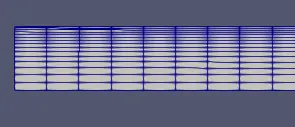
Now in the openFoam when we take paraFoam we get the mesh
side view:-
Front view:-
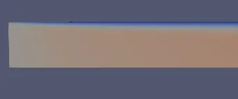
Velocity effect:-
at inlet
at outlet
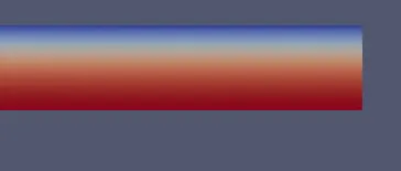
So we can see from the above pictures that the velocity is zero at the boundary of the pipe (No slip condition). The velocity is 0.1 m/s at the begining and increases wrt z and at the end of the pipe it will be maximum.
Pressure effect:-
at inlet

at outlet

We can see from the figures that the pressure is high at the inlet and at the end of the pipe the pressure is zero. Because we have given the pressure to be zero at the boundary.
Residual Graph
To get the residual graph we need to give the 'foamMonitor -l postProcessing/residuals/0/residuals.dat' command. And we will get the following graph:- 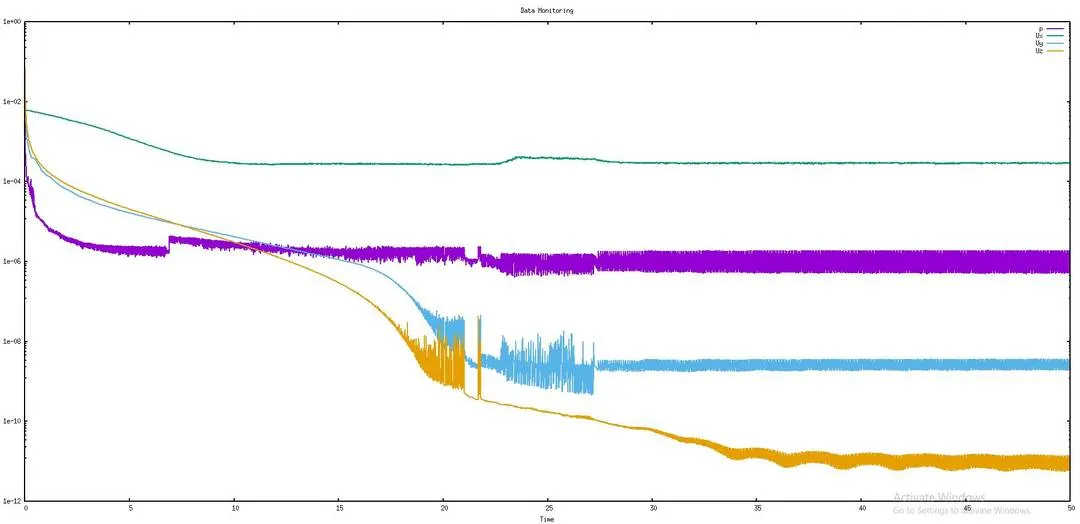
So from the graph we can say that the values become constant after a certain time period. So we can say that we get the convergent results. It goes to the steady state condition.
Now when we execute the matlab program we get the following graph:-
Velocity profile at different points
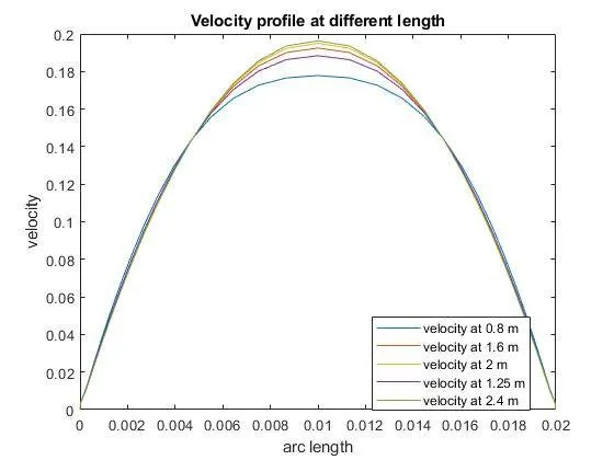
So we can see from the graph that initially the velocity profile doesn't fully develop. When we go near the hydrodynamic entrance length it starts to fully develop and at the hydrodynamic entrance length it developed fully and after that it does not change.
Analytical and Numerical Velocity comparison
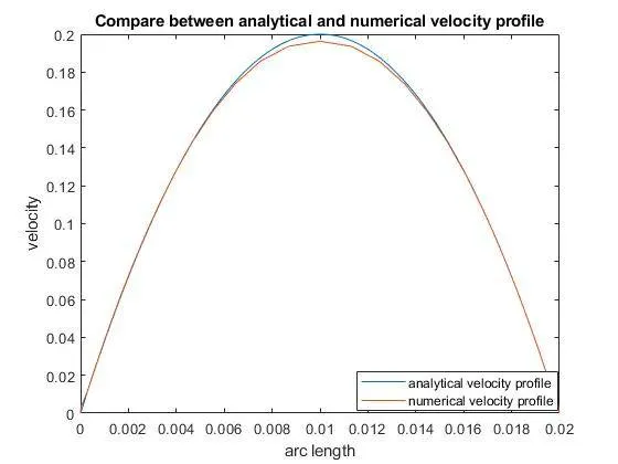
We can see from the graph that numerically we get almost the same values as the analytically calculated velocity. There is a minor difference between both of them. So we can say that we get the converged result.
Analytical and Numerical Shear Stress comparison
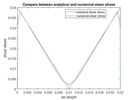
We can see from the graph that numerically we get almost the same values as the analytically calculated shear stress. There is a minor difference between both of them. So we can say that we get the converged result.
Analytical and Numerical pressure drop comparison
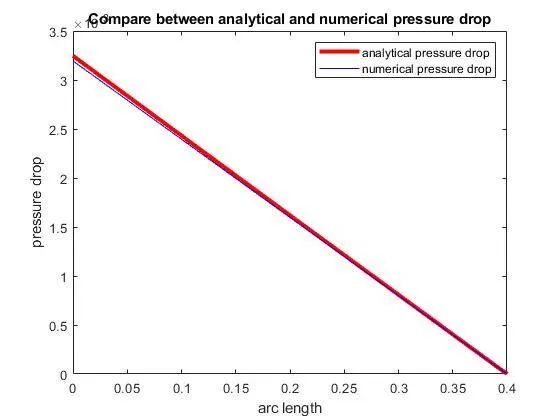
We can see from the graph that numerically we get almost the same values as the analytically calculated pressure. There is a minor difference between both of them. So we can say that we get the converged result.
Comparison of the results
| Velocity (max) | Shear Stress (max) | Pressure drop (2.1 t0 2.5 m) | |
| Analytical Solution | 0.20 | 0.0399 | 0.0032 |
| Numerical Solution | 0.196338 | 0.0378 | 0.0031 |
| Error % | 1.831 | 5.26 | 3.125 |
So we can say that we get a very small error%. The result we got is almost same as the actual values.