Project 2 - Rankine cycle Simulator

Code:- In this program we are going to plot rankine cycle and we are going to calculate the efficiency of the rankine cycle. In this program we are going to extract the values from the Xsteam function.

Rankine Cycle is a process which is mostly use in power plant to check the performance of the turbine. Code for this program:-

clear all
close all
clc


% user inputs 
p1 = input('Turbine Inlet Pressure(in bar):');
t1 = input('Turbine Inlet temperature(in degree celcius):');
p2 = input('Turbine Outlet Pressure or  Condenser Inlet Pressure(in bar):');

%state variable at point 1
s1 = XSteam('s_pT',p1,t1);
h1 = XSteam('h_pT',p1,t1);

%state variable at point 2
s2 = s1;
sf2 = XSteam('sL_p',p2);
sg2 = XSteam('sV_p',p2);

% s2 = sf2 + x2(sg2-sf2)
x2 = (s2-sf2)/(sg2-sf2);

hf2 = XSteam('hL_p',p2);
hg2 = XSteam('hV_p',p2);
% h2 = hf2 + x2(hg2-hf2)
h2 = hf2+(x2*(hg2-hf2));
p3 = p2;
t3 = XSteam('Tsat_p',p3);
t2 = t3;
% state variable at point 3
p3 = p2;

h3 = XSteam('hL_p',p3);
s3 = XSteam('sL_T',t3);


% state variable at point 4
p4 = p1;
s4 = s3;
h4 = XSteam('h_ps',p4,s4);
cp4 = XSteam('Cp_ph',p4,h4);
cv4 = XSteam('Cv_ph',p4,h4);
% gamma
ga = cp4/cv4;
k = (ga-1)/ga;
% p3v3^ga = p4v4^ga
%v3/v4 = (p4/p3)^(1/ga)
% p3v3/t3 = p4v4/t4
% t4/t3 = (p4/p3)*(p3/p4)^(1/ga)
% t4/t3 = (p4/p3)^((ga-1)/ga)
t4 = t3*(p4/p3)^k;

h5 = XSteam('hL_p',p4);
s5 = XSteam('sL_p',p4);
t5 = XSteam('Tsat_p',p4);

h6 = XSteam('hV_p',p4);
s6 = XSteam('sV_p',p4);
t6 = XSteam('Tsat_p',p4);

%calculation
% pump work
w_p = h4-h3
%heat addition
Q_a = h1-h4
%turbine work
w_t = h1-h2
%heat rejection
Q_r = h2-h3
% net work
W = w_t-w_p
%efficiency
N = (W/Q_a)*100
% back work ratio
r_bw = w_p/w_t


T = linspace(1,377,400);
for i = 1:length(T)
    hg(i) = XSteam('hV_T',T(i));
    hf(i) = XSteam('hL_T',T(i));
    sg(i) = XSteam('sV_T',T(i));
    sf(i) = XSteam('sL_T',T(i));
   
end

% plotting
figure(1)
hold on
plot(sf,T,'color','r')
plot(sg,T,'color','r')

text(s1,t1,'1')
text(s2,t2,'2')
text(s3,t3,'3')
text(s4,t4,'4')
plot(s5,t5,'*')
plot(s6,t6,'*')
plot([s1 s2 s3 s4 s5 s6 s1],[t1 t2 t3 t4 t5 t6 t1],'color','b')
xlabel('Entropy')
ylabel('Temprature')

figure(2)
hold on
plot(sf,hf,'color','r')
plot(sg,hg,'color','r')
text(s1,h1,'1')
text(s2,h2,'2')
text(s3,h3,'3')
text(s4,h4,'4')
plot(s5,h5,'*')
plot(s6,h6,'*')
plot([s1 s2 s3 s4 s5 s6 s1],[h1 h2 h3 h4 h5 h6 h1],'color','b')
xlabel('Entropy')
ylabel('Enthalpy')
    

Steps:- To make the program following steps I have taken:-

Step-1:- First we are going to give the needed inputs. We want program to run on the user inputs. So we are going to use 'input' command. So we are going to need three values as input. Which are the pressure and temprature at turbine inlet(p1 & t1) and pressure at turbine outlet(p2).

p1 = input('Turbine Inlet Pressure(in bar):');
t1 = input('Turbine Inlet temperature(in degree celcius):');
p2 = input('Turbine Outlet Pressure or Condenser Inlet Pressure(in bar):');

Step-2:- Now we are going to get the values of enthalpy and entropy at state-1. In order to do that we are going to use 'XSteam' function which we have given already.

s1 = XSteam('s_pT',p1,t1);:- This is to get the value of Entropy with the pressure and temprature values at p1 and t1 as input.
h1 = XSteam('h_pT',p1,t1);:- This is to get the value of Enthalpy with the pressure and temprature values at p1 and t1 as input.

Step-3:- Now we are going to get the values at state-2. Process 1-2 is 'Isentropic Expansion Process'. In the Isentropic Expansion Process there is no heat transfer that's why the value of the entropy does not change in this process. So entropy at point 2 is going to be same as point 1 value. 's2 = s1'

Now we need to check that point 2 is in which state. In order to do that we are going to check the dryness factor. To calculate that we are going to need the entropy at saturated liquid point and saturated vapour point at pressure p2.

sf2 = XSteam('sL_p',p2);:- This is to get the value of Entropy with the pressure at saturated liquid point at pressure p2.
sg2 = XSteam('sV_p',p2);:- This is to get the value of Entropy with the pressure at saturated vapour point at pressure p2.

Now we can calculate the dryness factor. '`x_2 = (s_2-s_(f2))/(s_(g2)-s_(f2))`'

Now we can calculate the enthalpy at point 2. so we are gonna need the enthalpy at saturated liquid point and saturated vapour point at pressure p2.

hf2 = XSteam('hL_p',p2);:- This is to get the value of Enthalpy with the pressure at saturated liquid point at pressure p2.
hg2 = XSteam('hV_p',p2);:- This is to get the value of Enthalpy with the pressure at saturated vapour point at pressure p2.

So enthalpy at point 2 is '`h_2 = h_(f2)+(x_2*(h_(g2)-h_(f2))`'

Step-4:- Now we know that the state 3 is at saturated liquid curve and the temprature at state 2 and 3 are equal. So in order to calculate the temprature at point 2 first we are going to calculate the temprature at state 3.

Process 2-3 is constant pressure process so 'p3 = p2'.

So to get the temprature at point 3. 't3 = XSteam('Tsat_p',p3);':-This is to get the value of temprature with the pressure at point 3.

So temprature at point 2. 't2 = t3'

Now we can get the enthalpy and entropy at point 3.

h3 = XSteam('hL_p',p3);:- This is to get the value of Enthalpy with the pressure at saturated liquid point at pressure p3.
s3 = XSteam('sL_T',t3);:- This is to get the value of Entropy with the temprature at saturated liquid point at temprature t3.

Step-5:- Now we are going to calculate the values at state 4.

Process 4-1 is a 'constant pressure process'. So pressure is constant. 'p4=p1'

Process 3-4 is an 'isentropic compression process'. So entropy is not going to change. So 's4=s3'

h4 = XSteam('h_ps',p4,s4);:- This is to get the value of Enthalpy with the pressure and entropy values at p4 and s4 as input.

Now to calulate the temprature at point 4 to do that we are going to need some values. We are going to use 'isentropic relation' and perfect gas law to calculate the temprature at point 4. So in process 3-4

`p_3*v_3^gamma = p_4*v_4^gamma`

`v_3/v_4 = (p_4/p_3)^(1/gamma)`

and gas law= `p_3*v_3/t_3 = p_4*v_4/t_4`

`t_4/t_3 = (p_4/p_3)*(p_3/p_4)^(1/gamma)`

`t_4 = t_3*(p_4/p_3)^((gamma-1)/gamma)`

So we have all the values at state-4

Step-6:- Process 4-1 is a constant pressure heat addition process. So during this process the pressure remains same. But state of the water changes. It goes from liquid to vapour state. So in the process the curve of process 4-1 cuts the saturation curve two times first at saturated liquid curve(point-5) second time at saturated vapour curve(point-6) than it goes to the superheated state at point 1. So we are going to need these two point to show them in our curve.

At point 5:-

h5 = XSteam('hL_p',p4);:- This is to get the value of Enthalpy with the pressure at saturated liquid point at pressure p4.
s5 = XSteam('sL_p',p4);:-This is to get the value of Entropy with the pressure at saturated liquid point at pressure p4.
t5 = XSteam('Tsat_p',p4);:-This is to get the value of temprature with the pressure p4 at saturated liquid curve.

At point 6:-

h6 = XSteam('hV_p',p4);:- This is to get the value of Enthalpy with the pressure at saturated vapour point at pressure p4.
s6 = XSteam('sV_p',p4);:-This is to get the value of Entropy with the pressure at saturated vapour point at pressure p4.
t6 = XSteam('Tsat_p',p4);:-This is to get the value of temprature with the pressure p4 at saturated liquid curve.

Step-7:- Now we are going to calulate the work, heat, efficiency and back work ratio of the rankine cycle.

In the rankine cycle work is done on the system by the pump. It is an input work. So pump work is nothing but the enthalpy change due to pump on the system ( difference between enthalpy at pump input to enthalpy at pump output).

`w_p = h_4-h_3`

Heat addition occurs in the boiler. So we can calculate that by calculate enthalpy difference in the boiler.

`Q_a = h_1-h_4`

In the rankine cycle we get the output by the turbine. So the turbine work is calculated by difference between enthalpy at turbine input to enthalpy at turbine output.

`w_t = h_1-h_2`

Heat rejection occurs in the condenser. So we can calculate that by calculate enthalpy difference in the condenser.

`Q_r = h_2-h_3`

The net work is done by the system is the difference of work input and work output.

`W = w_t-w_p`

Now we are going to calculate the efficiency of the cycle. It is the ratio of output and input.

`N = (W/Q_a)*100`

Now we are going to calculate the back work ratio. It is the ratio of input work and output work.

`r_(bw) = w_p/w_t`

Step-7:- Now we are going to plot t-s and h-s graph with the saturation curve graph.

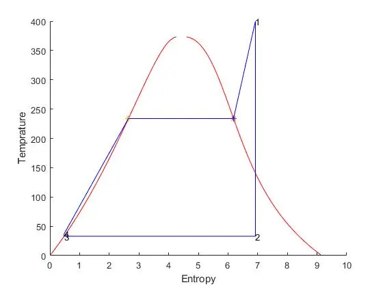
In figure(1) we are going to plot T-S graph and saturation curve. So we are going to need the every point of saturated liquid curve and saturated vapour curve.

For that we are going to use 'for loop'. We are going to get the enthalpy and entropy at temprature from 1 to 377 for saturated liquid and saturated vapour.

hf(i) = XSteam('hL_T',T(i));:-This is to get the value of Enthalpy with the temprature at saturated liquid point at temprature T.
hg(i) = XSteam('hV_T',T(i));:--This is to get the value of Enthalpy with the temprature at saturated vapour point at temprature T.
sf(i) = XSteam('sL_T',T(i));:--This is to get the value of Entropy with the temprature at saturated liquid point at temprature T.
sg(i) = XSteam('sV_T',T(i));:--This is to get the value of Entropy with the temprature at saturated vapour point at temprature T.

Now to plot that we are going to use plot command to plot the entropy w.r.t. temprature. 'plot(sf,T,'color','r')'

Now to plot that we are going to use plot command to plot the entropy w.r.t. temprature. 'plot(sg,T,'color','r')'

We want to indicate the state in the curve so we are going to use 'text' command to do that. 'text(x,y,'text')'

And point 5 and point 6 is going to be marked by marker '*'.

Now we are going to join all the 6 points with the help of 'plot' command.

We have given the axis name with 'label' command.

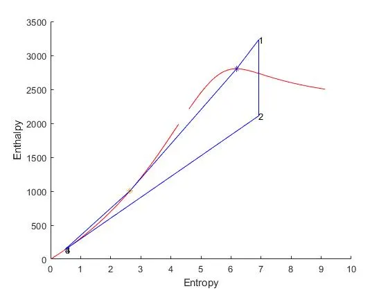
Step-8:- In figure(2) we are going to plot H-S graph and saturation curve. So we are going to need the every point of saturated liquid curve and saturated vapour curve.

Now to plot that we are going to use plot command to plot the enthalpy w.r.t. entropy. 'plot(sf,hf,'color','r')'

Now to plot that we are going to use plot command to plot the enthalpy w.r.t. entropy. 'plot(sg,hg,'color','r')'

We want to indicate the state in the curve so we are going to use 'text' command to do that. 'text(x,y,'text')'

And point 5 and point 6 is going to be marked by marker '*'.

Now we are going to join all the 6 points with the help of 'plot' command.

We have given the axis name with 'label' command.

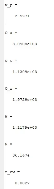
Output:- When we execute the program. It's going to ask the p1, t1 and p2 values.

I have given p1 = 30, t1 = 400 and p2 = 0.05.

So after giving the inputs it calculate the values and show in the command window.

We got the T-S graph with saturated curve. In the graph red curve is satured curve and blue line is rankine cycle process.

We get H-S graph with saturated curve. In the graph red curve is saturated curve and blue line is rankine cycle process.

Rankine Cycle:- Rankine cycle is mostly use in the power plant.

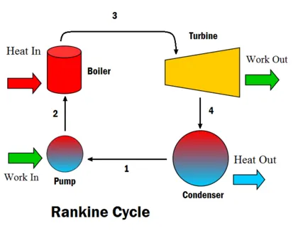
In the rankine cycle first pump pumps the water and increases the pressure of the water into the boiler. We gives heat to water in the boiler. The work of the boiler to convert the water into the steam. Than the steam is go to the turbine. And we get the work output. In the turbine the temprature of the steam is getting low. Noew the steam goes to the condenser. The work of the condenser to convert the steam into liquid form. In the condenser the heat is rejected. Now the water is again go into the pump from the condenser.