Week 4 - Genetic Algorithm

Code:- Code in MATLAB to optimise the stalagmite function and find the global maxima of the function. In order to do that we are going to use concept of Genetic Algorithm(GA). GA is a search-based optimisation technique based on the principles of genetics and natural selection.

clear all
close all
clc

%preparing the search space
x = linspace(0,0.6,150);
y = linspace(0,0.6,150);
%creating 2-D mesh
[xx yy] = meshgrid(x,y);
num_case = 50;

%evaluating the stalagmite function
for i = 1:length(xx)
    for j = 1:length(yy)
        input_vector(1)=xx(i,j);
        input_vector(2)=yy(i,j);
        f(i,j) = stalagmite(input_vector);
    end
end


% study-1 stastical behaviour
for i = 1:num_case
    [inputs,f_opt(i)]= ga(@stalagmite, 2);
    x_opt(i) = inputs(1);
    y_opt(i) = inputs(2);
end
f_opt = abs(f_opt);

%plotting
figure(1)
subplot(2,1,1)
hold on
surfc(x,y,abs(f))
shading interp
plot3(x_opt,y_opt,f_opt,'marker','o','markersize',5,'markerfacecolor','r')
title('unbounded inputs')
subplot(2,1,2)
plot(f_opt)
xlabel('iteration')
ylabel('function maximum')


% study-2 stastical behaviour with upper and lower bounds
for i = 1:num_case
    [inputs,f_opt(i)]= ga(@stalagmite, 2, [],[],[],[],[0;0],[0.6;0.6]);
    x_opt(i) = inputs(1);
    y_opt(i) = inputs(2);
end
f_opt = abs(f_opt);

%plotting
figure(2)
subplot(2,1,1)
hold on
surfc(x,y,abs(f))
shading interp
plot3(x_opt,y_opt,f_opt,'marker','o','markersize',5,'markerfacecolor','r')
title('bounded inputs')
subplot(2,1,2)
plot(f_opt)
xlabel('iteration')
ylabel('function maximum')


% study-3 stastical behaviour with increasing ga iteration
options = optimoptions('ga');
options = optimoptions(options,'populationsize',500);

for i = 1:num_case
    [inputs,f_opt(i)]= ga(@stalagmite, 2, [],[],[],[],[0;0],[0.6;0.6],[],[],options);
    x_opt(i) = inputs(1);
    y_opt(i) = inputs(2);
end
f_opt = abs(f_opt);

%plotting
figure(3)
subplot(2,1,1)
hold on
surfc(x,y,abs(f))
shading interp
plot3(x_opt,y_opt,f_opt,'marker','o','markersize',5,'markerfacecolor','r')
title('bounded inputs with modified iteration size')
subplot(2,1,2)
plot(f_opt)
xlabel('iteration')
ylabel('function maximum')

Steps:- To write this program I have taken the following steps:-

Step-1:- We need some input values to optimise the function. We are gonna need the search space. So we have taken two 1-D arrays.

x = linspace(0,0.6,150);
y = linspace(0,0.6,150);

From these we are going to make a 2-D array. To make this we are going to use 'meshgrid' command.

[xx yy] = meshgrid(x,y);

And we have taken the no. of cases to be 50.

Step-2:- Now we are going to evaluate the stalagmite function. We are going to use 'for loop' to generate the data for the plot. In the 'for loop' for each and every value of x and y we are creating an array name 'input_vector'. Now we are going to use 'stalagmite' function. Stalagmite function takes the 'input_vector' and calculate the f.

f(i,j) = stalagmite(input_vector);

Step-3:- Stalagmite function:- The fomula of the stalagmite is this:-

f = f1x*f2x* f1y*f2y

where f1x = (sin((5.1*pi)*input_vector(1)+0.5))^6;
f1y = (sin((5.1*pi)*input_vector(2)+0.5))^6;
f2x = exp(((input_vector(1)-0.0667)^2/0.64)*-4*log(2));
f2y = exp(((input_vector(2)-0.0667)^2/0.64)*-4*log(2));

We are going to use Genetic Algorithm which gives us the minimum optimisation. But we need the maximum value for our challenge. That's why I have taken the negegative value in the function. So that it will gives us the minimum value of f which is in actually maximum value of the function. So I have taken this "f = -f1x*f2x*f1y*f2y;".

function [f] = stalagmite(input_vector)

f1x = (sin((5.1*pi)*input_vector(1)+0.5))^6;
f1y = (sin((5.1*pi)*input_vector(2)+0.5))^6;
f2x = exp(((input_vector(1)-0.0667)^2/0.64)*-4*log(2));
f2y = exp(((input_vector(2)-0.0667)^2/0.64)*-4*log(2));
f = -f1x*f2x*f1y*f2y;

end

Step-4:- Now we are going to study the stastical behaviour for the unbounded inputs.

So in order to do that we are using 'for loop'. In the for loop we are calling the Genetic Algorithm "ga".

[inputs,f_opt(i)]= ga(@stalagmite, 2)

In the above command first we are giving the name of function which we need to be optimised and 2 is the no. of variable as input.

We are storing the optimum values of x, y and f in x_opt, y_opt and f_opt respectively.

So it will gives us the f_opt values in negative because we have calculated stalagmite value in negative in order to optimise maximum value. So now we need to convert this value in positive. So to do that we are going to use 'abs' command. It changes the value from negative to positive.

f_opt = abs(f_opt);

Step-5:- Now we are going to make plot. We are going to plot 2 graph in a single figure so we are going to use 'subplot' command.

• So in the figure first we plotting the surface plot. To do that we are using 'surfc' command. "surfc(x,y,abs(f))"
• We are using 'shading interp' which basically remove the grid lines from the plot. We use this command so that we can see the plot clearly.
• Now we are using the 'plot3' command to plot the optimise value of x, y and optimum function which 'ga' predict over the 50 studies. We are using 'marker' command to mark the optimise value in the plot with size 5 and face color of red. "plot3(x_opt,y_opt,f_opt,'marker','o','markersize',5,'markerfacecolor','r')".
• In the second sub plot we are going to plot the optimise value of the function."plot(f_opt)"
• We have given title to this figure is 'unbounded inputs'. "title('unbounded inputs')"
• Now given the label to the x and y axis.

Step-6:- Now we are going to study the stastical behaviour with upper and lower bounds.

So in order to do that we are using 'for loop'. In the for loop we are calling the Genetic Algorithm "ga".

[inputs,f_opt(i)]= ga(@stalagmite, 2, [],[],[],[],[0;0],[0.6;0.6]);

In the above command first we are giving the name of function which we need to be optimised, 2 is the no. of variable as input, now we have to give linear equalities which we don't have so we have use [],[],[],[]. Now we have to give the lower and upper range of the variable [0;0] is the lower range and [0.6;0.6] is the upper range.

We are storing the optimum values of x, y and f in x_opt, y_opt and f_opt respectively.

So it will gives us the f_opt values in negative because we have calculated stalagmite value in negative in order to optimise maximum value. So now we need to convert this value in positive. So to do that we are going to use 'abs' command. It changes the value from negative to positive.

f_opt = abs(f_opt);

Step-7:- Now we are going to make plot. We are going to plot 2 graph in a single figure so we are going to use 'subplot' command.

• So in the figure first we plotting the surface plot. To do that we are using 'surfc' command. "surfc(x,y,abs(f))"
• We are using 'shading interp' which basically remove the grid lines from the plot. We use this command so that we can see the plot clearly.
• Now we are using the 'plot3' command to plot the optimise value of x, y and optimum function which 'ga' predict over the 50 studies. We are using 'marker' command to mark the optimise value in the plot with size 5 and face color of red. "plot3(x_opt,y_opt,f_opt,'marker','o','markersize',5,'markerfacecolor','r')".
• In the second sub plot we are going to plot the optimise value of the function."plot(f_opt)"
• We have given title to this figure is 'bounded inputs'. "title('bounded inputs')"
• Now given the label to the x and y axis.

Step-8:- Now we are going to study the stastical behaviour with upper and lower bounds and with increasing ga iteration. By default 'ga' takes 50 values as the population. So instead of global minima it's find the local minima. So we are going to increase the population size to get the more accurate value. I have taken the population size to be 500.

options = optimoptions('ga');

It returns a set of default options for the solvername 'ga'.

Now we need population size to be 500 so we are going to use the following command:-

options = optimoptions(options,'populationsize',500);

Step-9:- Now we are going to use 'for loop'. In the for loop we are calling the Genetic Algorithm "ga".

[inputs,f_opt(i)]= ga(@stalagmite, 2, [],[],[],[],[0;0],[0.6;0.6],[],[]'options);

In the above command first we are giving the name of function which we need to be optimised, 2 is the no. of variable as input, now we have to give linear equalities which we don't have so we have use [],[],[],[]. Now we have to give the lower and upper range of the variable [0;0] is the lower range and [0.6;0.6] is the upper range.. Now we have to give nonlinear constraints which we don't have so we are using [],[]. Now we are using 'options' which changes the population size to be 500.

We are storing the optimum values of x, y and f in x_opt, y_opt and f_opt respectively.

So it will gives us the f_opt values in negative because we have calculated stalagmite value in negative in order to optimise maximum value. So now we need to convert this value in positive. So to do that we are going to use 'abs' command. It changes the value from negative to positive.

f_opt = abs(f_opt);

Step-10:- Now we are going to make plot. We are going to plot 2 graph in a single figure so we are going to use 'subplot' command.

• So in the figure first we plotting the surface plot. To do that we are using 'surfc' command. "surfc(x,y,abs(f))"
• We are using 'shading interp' which basically remove the grid lines from the plot. We use this command so that we can see the plot clearly.
• Now we are using the 'plot3' command to plot the optimise value of x, y and optimum function which 'ga' predict over the 50 studies. We are using 'marker' command to mark the optimise value in the plot with size 5 and face color of red. "plot3(x_opt,y_opt,f_opt,'marker','o','markersize',5,'markerfacecolor','r')".
• In the second sub plot we are going to plot the optimise value of the function."plot(f_opt)"
• We have given title to this figure is 'bounded inputs with modified iteration size'. "title('bounded inputs with modified iteration size')"
• Now given the label to the x and y axis.

Output:- When we execute the program it will calculate the optimum value of function and plot the surface with optimum value and optimum value in respect to iteration.

Figure(1):-

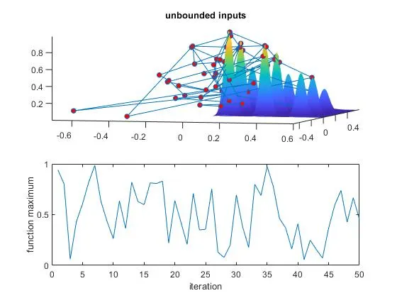
In this figure we can see that it gives us the f_opt value outside of the search space. It's happening because we haven't given the bounda to the program. We are getting optimise value outside the search space. The maximum value varies from 0 to 1. So it is not a good way to calculate the global maxima of the function.

Figure(2):-

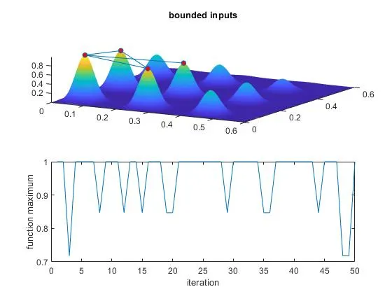
Now we are getting the more clear plot with more accurate optimise value. Because we have given the search range to the program. The maximum value varies from 0.7 to 1. Now we have the more clear plot with more accurate values. The function is prediciting that the maximum value of the function is in between the four peaks.

Figure(3):-

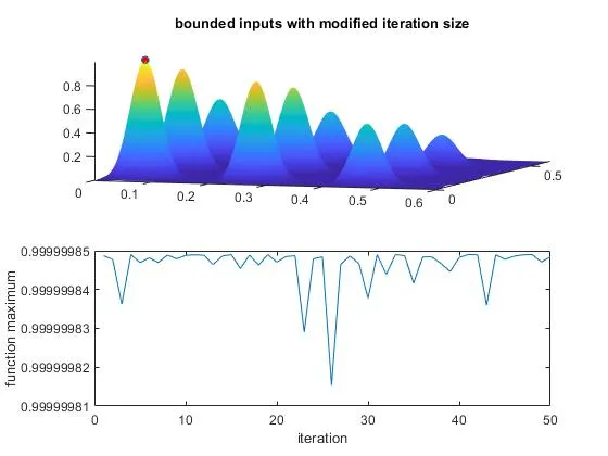
Now we are getting the more clear plot in compare to last one. because in the third study we have increases the population size with the bound range. In the plot we can clearly see the global maxima in a red color dot. So it gives us the best result in the all three cases. The function maximum value is nearly 1. so this is the best way to find the global maxima.

Concept of Genetic Algorithm:- Genetic Algorithm is a search-based optimisation technique based on the principles of genetics and natural selection. It uses in optimization problem. We can understand how GA works by this graph:-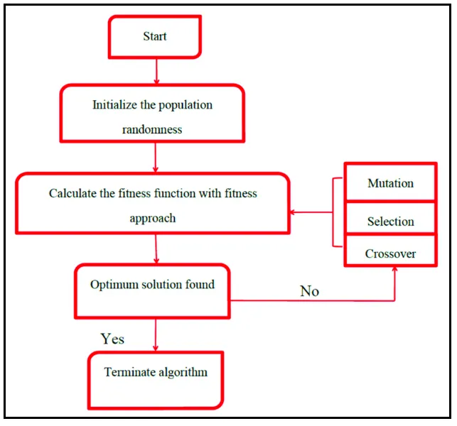

• GA process begins with a set of individuals which we called a population. Population is the no. of sample data takenon which the GA is perforemed.
• Now it select the parents from the population data. In the selection the main objective of the GA is to select the highly fit individual and let them pass their genes to the next generation
• Now it taken the cross-over process. In this process the parents which we have selected from the population mates and we got a child with a new gene(offspring).
• In new offsprings, some of them go to mutation. It means in order to get more accurate value. Some child go into the mutation so that we can get more accurate values.

Syntax:- Syntax for ga:-

1. x = ga(fun,nvars):- Finds a local unconstrained minimum, x, to the objective function, fun. nvars is the dimension (number of design variables) of fun.

2. x = ga(fun,nvars,A,b,Aeq,beq,lb,ub):- Find the minimum x, to the objective function, nvars is the dimension (number of design variables) of fun subject to the linear inequalities A*x ≤ b for the linear equalities Aeq*x = beq with upper and lower limit.

3. options = optimoptions(solvername):- Returns a set of default options for the SolverName solver.

4. options = optimoptions(options,name,value):- Returns options with the named parameters altered with the specified values.

5.x = ga(fun,nvars,A,b,Aeq,beq,lb,ub,nonlcon,options):- Find the minimum x, to the objective function, nvars is the dimension (number of design variables) of fun subject to the linear inequalities A*x ≤ b for the linear equalities Aeq*x = beq with upper and lower limit.nonlcon accepts x and returns vectors C and Ceq, representing the nonlinear inequalities and equalities respectively and optimization parameters replaced by values in options.