Week 5 - Curve fitting
Theory
Curve fitting is the procees of constructing a closet proximity to the real series of data. By curve fitting we can construct the functional relationship between observed dataset and parameter values.
(A) It help to carry out the system simulation and optimization.
(b) To determinate value at the intermidate point.
(c) To the trend analysis
- What does popt and pcov mean?
popt—it give the optimized value of coefficient that are used in the polynomial(defined function)
pcov—it gives covariance matrix of the 2D array of estimated popt. Diagonal of pcov gives the
variance of the parameter estimated(popt). It help to compute the standred deviation error of the
parameter (coefficent used in the defined function)
- What does np.array(temperature) do?
By this we can convert the float array into int type error, if would not do this then it will display
error can’t multiply float type value.
- What does the * in *popt mean?
Since popt is optimized array of the coefficient that are used in the defined function, so in order to
pass more than one value we need apply * notation.
4. Write code to fit a linear and cubic polynomial for the Cp data. Show empirically as to how well
our curve has been fit.
#LINEAR CURVE FIT
import numpy as np
import matplotlib.pyplot as plt
from scipy.optimize import curve_fit
# curve fit function
def func(t,a,b):
return a*t+b
# Reading thermodynamic data file
def read_file():
temperture=[]
cp=[]
for line in open('data','r'):
values=line.split(',')
temperture.append(float(values[0]))
cp.append(float(values[1]))
return[temperture,cp]
# main program
temperture,cp=read_file()
popt,pocv=curve_fit(func,temperture,cp)
#print(popt)
#print(pocv)
fit_cp=func(np.array(temperture),*popt)
plt.plot(temperture,cp,color='blue')
plt.plot(temperture,fit_cp,color='red')
plt.title("LINEAR CURVE FIT")
plt.legend(['Actual data','curve_fit'])
plt.xlabel('temperture[K]')
plt.ylabel('cp(J/kgK)')
plt.show() 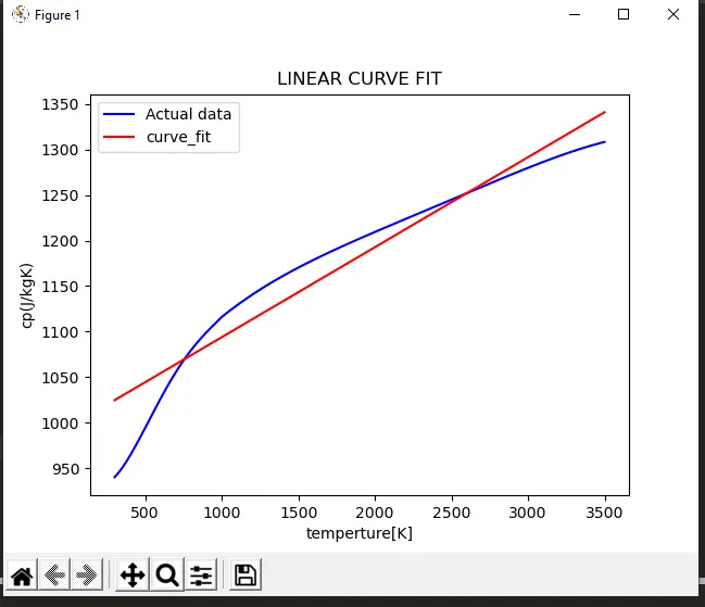 Procedure
1. imported all nesscery modules
2. Defined a function with arguments and first argument should always is independent variables then after the coefficent of desired function and later on this function will be used to find the best fit curve.
3. Then we defind a function to read the data, tempertre and cp are set as zero array so that we can store the tempertue and cp values with append command, comma notation used to distniguish between values, then we got 2D array that is "value"
4.Then i call the read_file function which consits the temperture and cp array. Becasue earlier it was inside the function only. Later it will used to get curve fit.
5. Obtained the curve fit with the help of scipy.optimize module.
6.Now we got curve fit so we need to calcute the value cp corresponding to obatined coefficents(*popt).
7.Then we plot graph with and naming with help of matplotlib module.
# cubic curve
import numpy as np
import matplotlib.pyplot as plt
from scipy.optimize import curve_fit
# curve fit function
def func(t,a,b,c,d):
	return pow(t,3)*a+pow(t,2)*b+c*t+d
# Reading thermodynamic data file
def read_file():
	temperture=[]
	cp=[]
	for line in open('data','r'):
		values=line.split(',')
		temperture.append(float(values[0]))
		cp.append(float(values[1]))
	return[temperture,cp]
# main program
temperture,cp=read_file()
popt,pocv=curve_fit(func,temperture,cp)
print(popt)
print(pocv)
fit_cp=func(np.array(temperture),*popt)
plt.plot(temperture,cp,color='blue')
plt.plot(temperture,fit_cp,color='red')
plt.title("CUBIC CURVE FIT")
plt.legend(['Actual data','curve_fit'])
plt.xlabel('temperture[K]')
plt.ylabel('cp(J/kgK)')
plt.show()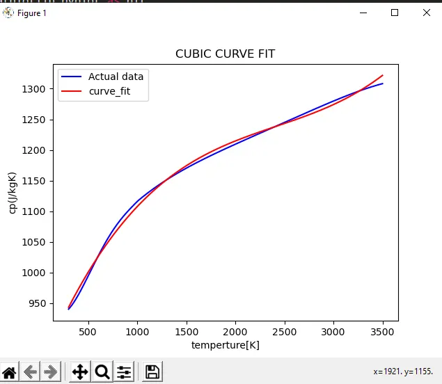
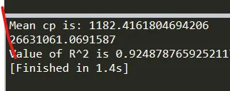
Calculation for good and bad curve
for linear curve
import numpy as np
import matplotlib.pyplot as plt
from scipy.optimize import curve_fit
def func(t,a,b):
	return a*t+b

def read_file():
	temp=[]
	cp=[]
	for line in open("data",'r'):
		value=line.split(',')
		temp.append(int(value[0]))
		cp.append(float(value[1]))
	return(temp,cp)
temp,cp=read_file()
popt,pocv=curve_fit(func,temp,cp)
fit_cp=func(np.array(temp),*popt)
#print(fit_cp)
#print(fit_cp[0])
#print(cp)
#print(cp[0])
#print(popt)
sum=0
"""

avg=np.sum(cp)/np.size(cp)
print(avg)
"""
n=1
"""
for i in range(len(cp)):
	sum=sum+cp[i]
	n=n+1
	#print(sum)
"""
for i in cp:
	n=n+1
	sum=sum+i

#print(n)
avg=sum/n

print("Mean cp is:",avg)

#print(cp)
SSR=0

for t in range(0,np.size(cp)):
	SSR=SSR+pow((fit_cp[t]-avg),2)
print(SSR)
SSE=0
#F=np.size(cp)
#print(F)

for j in range(0,np.size(temp)):
	SSE=SSE+pow((cp[j]-fit_cp[j]),2)

#print(SSE)
Rsqure=SSR/(SSE+SSR)
print('Value of R^2 is',Rsqure)
"""
SST=0
for k in range(0,np.size(cp)):
	SST=SST+pow((cp[k]-avg),2)
Rsqure=SSR/(SST)
print('Value of R^2 is',Rsqure)
"""
For cubic curve
import numpy as np
import matplotlib.pyplot as plt
from scipy.optimize import curve_fit
# curve fit function
def func(t,a,b,c,d):
	return pow(t,3)*a+pow(t,2)*b+c*t+d
# Reading thermodynamic data file
def read_file():
	temperture=[]
	cp=[]
	for line in open('data','r'):
		values=line.split(',')
		temperture.append(float(values[0]))
		cp.append(float(values[1]))
	return[temperture,cp]
# main program
temperture,cp=read_file()
popt,pocv=curve_fit(func,temperture,cp)
fit_cp=func(np.array(temperture),*popt)
n=1
"""
for i in range(len(cp)):
	sum=sum+cp[i]
	n=n+1
print(sum)
print(n)
avg=sum/n
print("Mean cp  is:",avg)
z=0
"""
avg=np.sum(cp)/np.size(cp)
SSR=0

for t in range(0,np.size(cp)):
	SSR=SSR+pow((fit_cp[t]-avg),2)
print(SSR)
SSE=0
#F=np.size(cp)
#print(F)
"""
for j in range(0,np.size(cp)):
	SSE=SSE+pow((cp[j]-fit_cp[j]),2)

print(SSE)
Rsqure=SSR/(SSE+SSR)
print('Value of R^2 is',Rsqure)
"""
SST=0
for k in range(0,np.size(cp)):
	SST=SST+pow((cp[k]-avg),2)
print(SST)
Rsqure=SSR/(SST)
print('Value of R^2 is',Rsqure)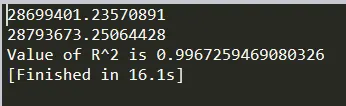
From the above R^2 value it is clear that cubic curve is the best curve fit because its R^2 value is more nearer to the one.
5. What needs to be done in order to make the curve fit perfect?
As we increse the order of polynomial it lead to decrese the error difference between ground truth value and fitted function, but incresing the order of polynomial doesnt help always, then we have to hit and trail on data points, according to data points we can have different different best curve fit on some portion of data points. We can change function and scaling and centering is also helpful.