Week 3 - Solving second order ODEs

Aim

1) Write a program in Python that will simulate the pendulum motion 0-20 sec, for angular displacement=0,angular velocity=3 rad/sec at time t=0.

2) create the animation of above pendulam motion

Theory

A pendulam consist of a ball(m) and a string. The string is connected to ball and to nail (hinge point), the weight of ball is due to gravity is mg and here we are assuming the string is massless. When we give some initial angular velocity from the equilibrium position(mid) to bob(m), then it produce the to and fro motion. When one cycle is complete (from extreme opposite points) by bob is called time period. After some time due to friction it will stop.

Equation of motion of pendulam

ma + bv +(gm/l)sinҨ = 0

a(accerlation)= d²Ҩ/dt

v(velocity)= dҨ/dt

length of string is l

g is accerlation due gravity, m is mass of ball

Ҩ is angular displacement

All unit in S.I

b is damping

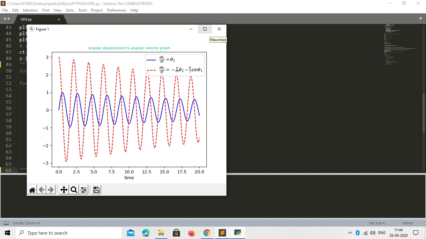
After solving the ODE we will get the angular displacements and angular velocities

Code

import numpy as np 
from scipy.integrate import odeint
import matplotlib.pyplot as plt 
import math
# function that returns
def model(theta,t,b,g,l,m):
	
	theta1=theta[0]
	theta2=theta[1]
	dtheta1_dt=theta2
	dtheta2_dt=-(b/m)*theta2-(g/l)*math.sin(theta1)
	dtheta_dt=[dtheta1_dt,dtheta2_dt]
	return dtheta_dt

# length of the string in m
l=1
# bob is at mean position and angular velocity(w) 3 rad/sec
t=0
theta=0
w=3
# coordinates of string hinge
x0=0
y0=0
# descrption of pendulam
b=0.05
g=9.81
m=1

# intial condition
ic=[0,3]
# time steps
t=np.linspace(0,20,400)

# solve the ODE
thetaa=odeint(model,ic,t,args=(b,g,l,m))

# plot results
plt.plot(t,thetaa[:,0],'b-',label=r'$\frac{d\theta_1}{dt}=\theta_2$')

plt.plot(t,thetaa[:,1],'r--',label=r'$\frac{d\theta_2}{dt}=-\frac{b}{m}\theta_2-\frac{g}{l}sin\theta_1$')

plt.title("angular displacement & angular velocity graph",fontsize=8,color='c')
plt.xlabel('time')
plt.legend(loc='best')
plt.show()
# coordinates of string end point where the bob is connected (x1,y1)
ct=1
z=[]
for i in thetaa[:,0]:
	z.append(i)
for theta in z:
	x1=-(x0+l*math.sin(theta))
	y1=-(y0+l*math.cos(theta))
	
	filename='test%05d.png'%ct
	ct=ct+1

	plt.figure()
	plt.plot([x0,x1],[y0,y1],'g')
	plt.plot([x1],[y1],'co',markersize=30)
	plt.title("pendulam motion",fontsize=15,color='g')
	plt.xlim([-1,1])
	plt.ylim([-2,1])
	plt.savefig(filename)

Procedure

• Imported all nesscery modules
• Defined a function (model) with arguments is theta,t,b,g,l,m.

Ҩ₁=Ҩ[0]

Ҩ₂=Ҩ[1]

dҨ₁/dt= Ҩ₂

dҨ₂/dt=-(b/m)*Ҩ₂-(g/l)*math.sin(Ҩ₁)

this is done to create the second order DE into ODE. Then make the matrix of

(dthetaa/dt)=([Ҩ₁,Ҩ₂]----(1)

similarly for right hand side also. Hence we will get required matrix.

• Then assign all given parameter.
• Define the initial conditions i.e angular displacement and angular velocity.
• Created the time array between 0 to 20 sec with 400 time steps to integrate ODE by odeint function by linspace command with help of numpy module
• Odeint is a function to integrate the differential equations(model) with help of scipy module and it gives the matrix (1)
• Plotted the graph between
• 1. Time array and angular displacement
  2. Time array and angular velocity

  With help of matplotlib.lib module

• Defined the string origin, for loop is applied to get the x1 and y1 corresponding to every angular displacement as the course of time.

• gave title of graph with help plt.title command, to differentiate between two curves legend is used.

• To show the graph plt.show()

• Different filename given to every bob position and having png extension, with the help of str(varaiable) command

• figure – create the each figure at different paper.

• Plotted the one metre length string in green color

• Created the circle with help markers.

• Fix the origin with help of x and ylim

• Finely save the different figure and display it.

• To make the animation magick *.png output.gif is used.

Result

It is evident from angular displacement and angular velocity plot as the time passes due damping amplitude of above mention term got decreased

Errors

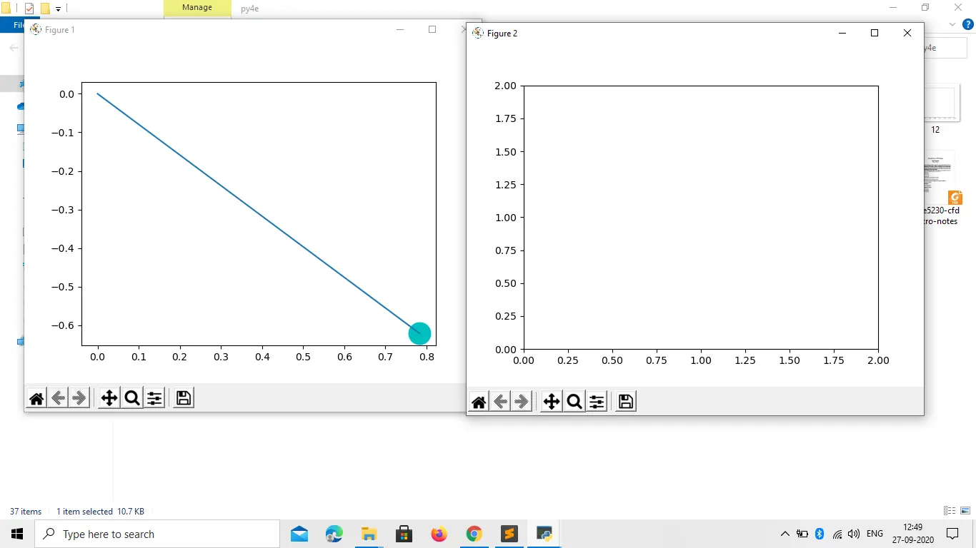
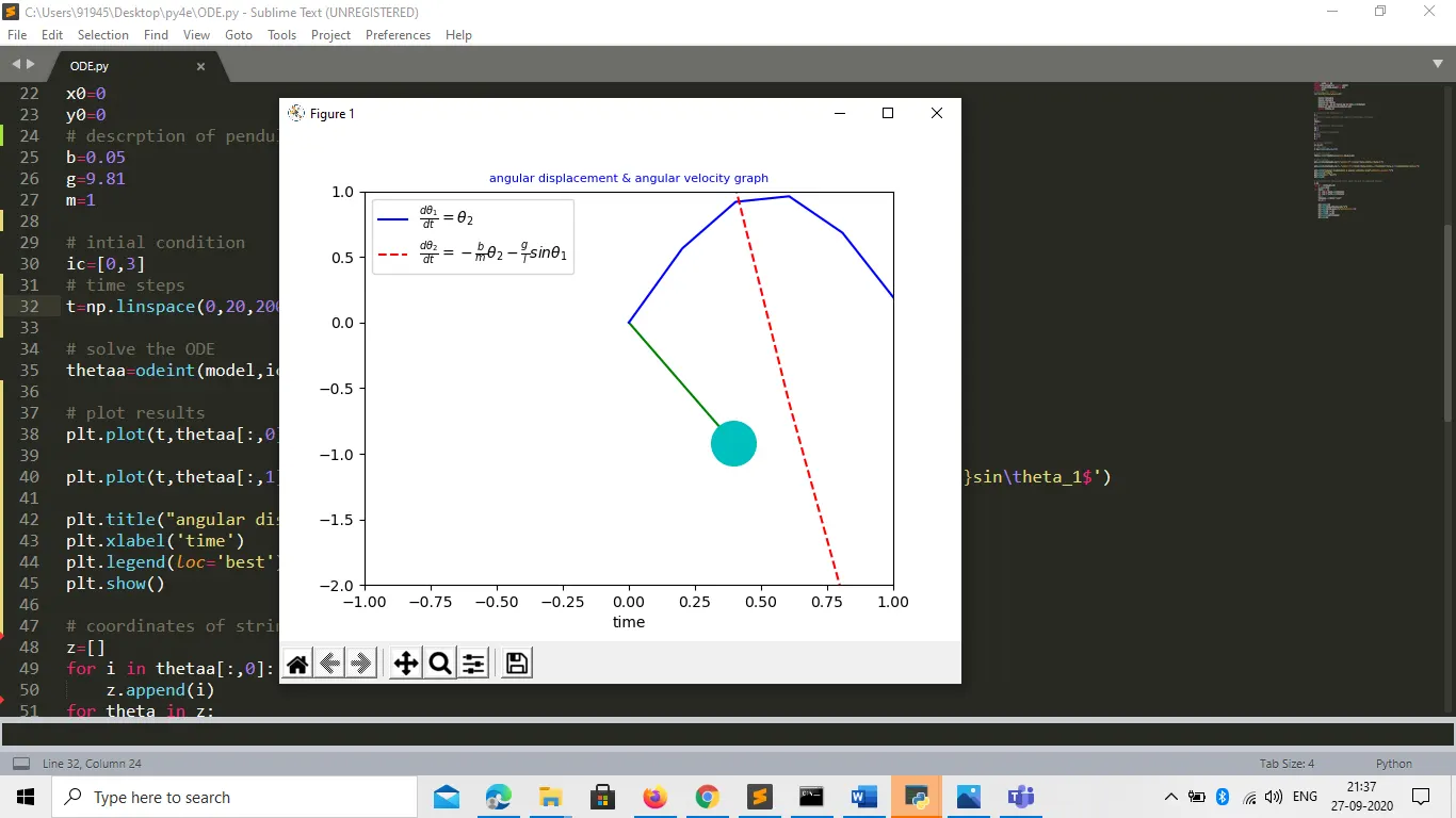
1) because of not proper x and ylim

2)by keeping the first plot(angular velocity and displacement) then after motion of pendulm plot with proper indentation.

animation link
https://www.youtube.com/watch?v=e32EDgdYklU