Week 3.5 - Deriving 4th order approximation of a 2nd order derivative using Taylor Table method

Central differencing

Number of nodes=order of derivative+order of approximation-1

=2+4-1=5

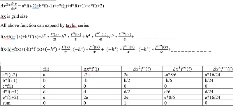
a+b+c+d+e=0

-2a-b+0+d+2e=0

2a+b/2+0+d/2+2e=1

-a*8/6-b/6+0+d/6+e*8/6=0

a*16/24+b/24+0+d/24+e*16/24=0

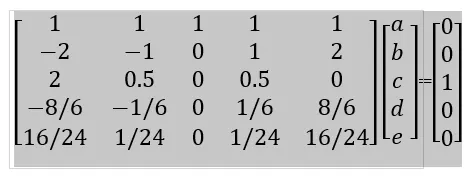
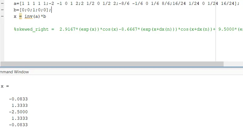
To get the value of the coefficients we can write in the matrix ie

AX=B

Skewed right side differencing

Number of nodes=order of derivative+order of approximation

=2+4=6

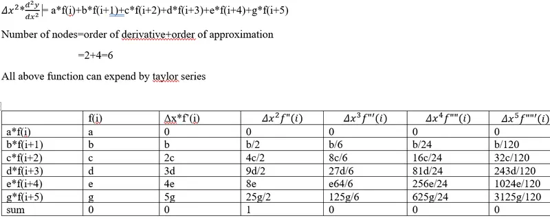
a+b+c+d+e+g=0

0+b+2c+3d+4e+5g=0

0+b/2+4c/2+9d/2+8e+25g/2=1

0+b/6+8c/6+27d/6+e64/6+125g/6=0

0+b/24+16c/24+81d/24+256e/24+625g/24=0

0+b/120+32c/120+243d/120+1024e/120+3125g/120=0

To get the value of the coefficients we can write in the matrix ie

AX=B

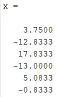
Skewed Left side differencing

Number of nodes=order of derivative+order of approximation

=2+4=6

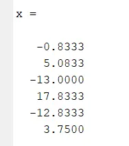
Similar to the right side skewed for further calculation, here all the coeifficient will remain for each nodes same because we are finding the solution in opposite direction.

% Main Program
close all
clear all
clc

x = pi/3;
dx=linspace(pi/4000,pi/4,200);

for n=1:200
% f(x) =(e^x)*cosx
% 2nd derivative ie f"(x) is
   Analytical_derivative = -(2*(exp(x)*sin(x)))
 
% Central difference of 2nd order derivative with 4th order accuracy(approximation)
%f(i-2) = (exp(x-2*dx))*cos(x-2*dx)
%f(i-1) = (exp(x-dx))*cos(x-dx)
%f(i) = (exp(x))*cos(x)
%f(i+2) = (exp(x+2*dx))*cos(x+2*dx)
%f(i+1) = (exp(x+dx))*cos(x+dx)
%numerical_derivative =
%-0.0833*f(i-2)+1.333*f(i-1)-2.5*f(i)+1.333*f(i+1)-0.0833*f(i+2)/dx^2
central_differencing = (((-0.083333333333333333333333333*((exp(x-(2*dx(n))))*(cos(x-(2*dx(n))))))+(1.3333333333333333333333333*((exp(x-dx(n)))*(cos(x-dx(n)))))-(2.5*((exp(x))*(cos(x))))+(1.333333333333333333333333333333*((exp(x+dx(n)))*(cos(x+dx(n)))))-(0.083333333333333333333333333333333*((exp(x+(2*dx(n))))*(cos(x+(2*dx(n)))))))/(dx(n)^2));
C_error(n) = abs(central_differencing- Analytical_derivative)

% Skewed right sided difference 2nd order derivative with 4th order accuracy(approximation)
%skewed_right = 3.75*f(i)-12.8333*f(i+1)+17.833*f(i+2)-13*f(i+3)+5.0833*f(i+4)-0.8333*f(i+5)
skewed_right = ((3.75*((exp(x))*(cos(x))))-(12.83333333333333333333*((exp(x+(dx(n))))*(cos(x+(dx(n))))))+(17.83333333333333333*((exp(x+(2*dx(n))))*(cos(x+(2*dx(n))))))-(13*((exp(x+(3*dx(n))))*(cos(x+(3*dx(n))))))+(5.08333333333333333333333*((exp(x+(4*dx(n))))*(cos(x+(4*dx(n))))))-(0.8333333333333333333333333*((exp(x+(5*dx(n))))*(cos(x+(5*dx(n)))))))/(dx(n)^2);
R_error(n) = abs(skewed_right- Analytical_derivative)

% Skewed right sided difference 2nd order derivative with 4th order accuracy(approximation)
skewed_left = (((-0.833333333333333333333333333*((exp(x-(5*dx(n))))*(cos(x-(5*dx(n))))))+(5.08333333333333333333333333333*((exp(x-(4*dx(n))))*cos(x-(4*dx(n)))))+(-13*((exp(x-(3*dx(n))))*cos(x-(3*dx(n))))))+(17.833333333333333333333333333*((exp(x-(2*dx(n))))*(cos(x-(2*dx(n))))))-(12.833333333333333333333333333333333*((exp(x-dx(n)))*cos(x-dx(n))))+(3.75*((exp(x))*cos(x))))/(dx(n)^2);
L_error(n) = abs(skewed_left- Analytical_derivative)
end
%k = C_error
%l = R_error
loglog(dx,C_error)
hold on
loglog(dx,R_error)
hold on
loglog(dx,L_error)
legend('center diff','right skew','left skew')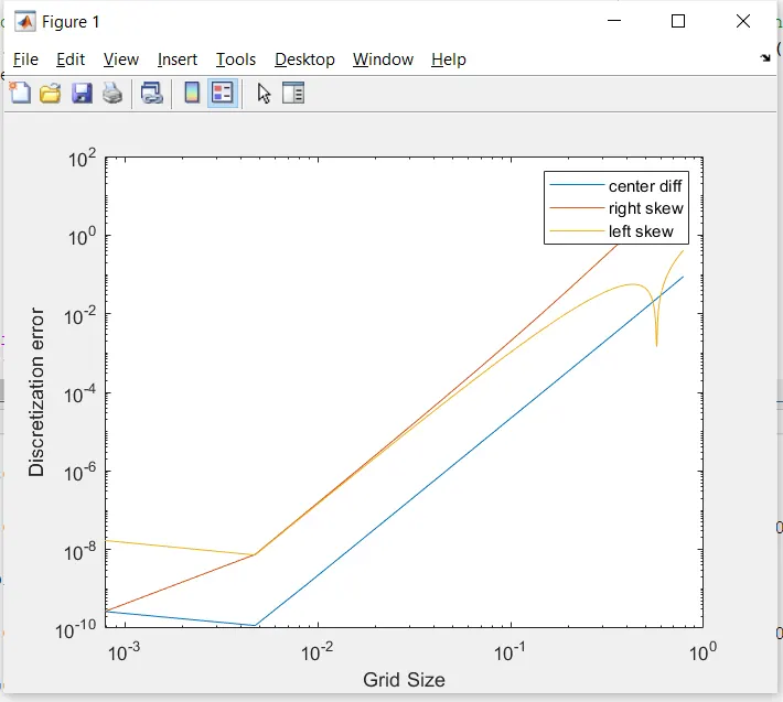

Result

As we can see the central differencing is showing less discritization error as compare to the SLSD and SRSD. This reason behind is that central differencing take the information form all neighbouring point of the reference point in both direction wheras other SLSD, SRSD take information in one direction only of the stencil

Why skewed scheme is useful.

In those sytem where information are available in one direction in that case skewed scheme has edge over the central differencing scheme.

What can a skewed scheme do that a CD scheme cannot?

Let suppose we have intial conditions at the boundary nodes then CDS cant be employed rather here skewed scheme will be very useful.