Week 2 Air standard Cycle

Aim- Write a program to print the pv diagram and thermal efficency of ideal otto cycle.

Theory- air standred cycle having following assumptions

1) air is the working fluid.

2) working fluid is the ideal gas.

3) specific heat values and gamma value are cosntant.

Since it is closed cycle the product of mass(m) and universal gas constant(R) is constant through out the cycle. Pressure(p1) and temperature (t1) are the conditions at the states point 1. After the heat addition at constant volume temperature rise to 2300 K and ratio of specific heat(gamma).

d= bore

l=stroke length

r_c=connecting rod

r= compression ratio

swept volume=sv

cv=clearance volume

all parameter are in S.I units.

It consist of four process

• Adiabatic compression(1-2) , pv^gamma=constant
• Heat addition at const. volume(2-3), v=constant
• Adiabatic expension(3-4), pv^gamma=constant
• Heat rejection at const. volume(4-1), v=constant

  Procedure

  • Calculated all parameter at all states points that is 1,2,3,4.
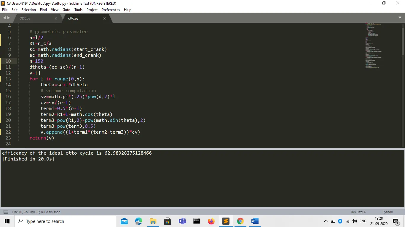
  • Define a function that is engine_kinematics(arguments) to get the relation of volume w.r.t theta, corresponding to that pressure variation can be find. It is applied on process 1-2 when crank move from BDC to TDC and 3-4 when crank move from TDC to BDC. Then for loop is applied with variable i and it runs 100 times and it gives 100 theta values. Then all volumes corresponding to 100 theta values stored in a array.

  V=(1+0.5*(r-1)(R1+1-cos(theta)-(R1)²(sin²(theta))^0.5)cv

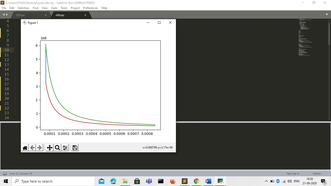
  PV diagram is plotted

  • straight line is plotted for process 2-3 and 4-1.
  • Exponential curve is plotted for remaining process.
  • Efficiency is calculated

  j=(1-(1/r^gamma-1)*100

  import math
  import matplotlib.pyplot as plt
  def engine_kinmeatics(d,l,r_c,r,start_crank,end_crank):
  
  	# geometric parameter
  	a=l/2
  	R1=r_c/a
  	sc=math.radians(start_crank)
  	ec=math.radians(end_crank)
  	n=100
  	dtheta=(ec-sc)/(n-1)
  	v=[]
  	for i in range(0,n):
  		theta=sc+i*dtheta
  		# volume computation
  		sv=math.pi*(.25)*pow(d,2)*l
  		cv=sv/(r-1)
  		term1=0.5*(r-1)
  		term2=R1+1-math.cos(theta)
  		term3=pow(R1,2)-pow(math.sin(theta),2)
  		term3=pow(term3,0.5)
  		v.append((1+term1*(term2-term3))*cv)
  	return(v)
  
  # input
  p1=101325
  t1=500
  t3=2500
  gamma=1.4
  # geometric parameter
  d=0.1
  l=0.1
  r_c=0.15
  r=8
  # volume computation
  sv=(math.pi/4)*pow(d,2)*l
  cv=sv/(r-1)
  v1=cv+sv
  # state point 2
  v2=cv
  # p2v2^gamma=p1v1^gamma
  p2=p1*pow(v1,gamma)/pow(v2,gamma)
  # p2v2/t2=p1v1/t1|rhs=mR/t1|mR=p2v2/t2
  mR=p1*v1/t1
  t2=p2*v2/mR
  v_compression=engine_kinmeatics(d,l,r_c,r,180,0)
  p_compression=[]
  for v in v_compression:
  	p_compression.append((p1*pow(v1,gamma))/pow(v,gamma))
  
  # state point 3
  v3=v2
  # p3v3/t3=p2v2/t2|rhs=p2v2/t2
  mR=p2*v2/t2
  p3=mR*t3/v3
  v_expension=engine_kinmeatics(d,l,r_c,r,0,180)
  p_expension=[]
  for v in v_expension:
  	p_expension.append((p3*pow(v3,gamma))/pow(v,gamma))
  
  # state point 4
  v4=v1
  # p4v4^gamma=p3v3^gamma
  p4=p3*pow(v3,gamma)/pow(v4,gamma)
  # p4v4/t4=mR
  t4=p4*v4/mR
  plt.plot([v2,v3],[p2,p3])
  plt.plot([v4,v1],[p4,p1])
  
  plt.plot(v_expension,p_expension)
  plt.plot(v_compression,p_compression)
  plt.show()
  # efficency(j)
  term4=pow(r,(gamma-1))
  j=(1-(1/term4))*100
  print("efficency of the ideal otto cycle is",j)

Result

1) Efficency is depends upon the compression ratio and gamma value. If we increse the compression ratio and gamma individual as well as simultenusly it leads to increase in efficency.

2) As we increase the maximum temperture of cycle area under pv diagram(work) is also increased but due to material constraints, it is not possible, along with it heat rejection rate is also increased.