Week 5.2 - Literature review: ODE Stability

Aim

To study and understand the concept of stability of ODE systems.

• When does an ODE become unstable?
• How does stability affect engineering simulations?
• Can stability condition be derived for all types of problems?

Introduction

We know that in CFD, we numerically simulate a physical system by solving its governing equations. These governing equations are either partial differential equations or ordinary differential equations. To solve these differential equations, we use various kinds of discretization schemes. However, not all discretization schemes may result in the correct or desired solution. The two factors that determine this choice are stability and consistency.

a) Stability: If the errors do not grow as the solution advances. If the residuals do not grow, the solution will eventually converge a steady state solution.

b) Consistency: If the solution approaches the actual analytical solution as the grid size approaches to zero. The error in a solution is directly proportional to the grid size. When the grid size tends to 0, the errors also should tend to zero and the solution also should tend to the analytical solution.

If a scheme satisfies both stability and consistency, then the solution is said to be converging i.e., it will reach a steady state, close to the desired physical result.

1. So, when does an ODE become unstable?

Let us understand the stability criteria for ODE using this general form of ODE

dy/dt = -ay

The analytical solution for this ODE is be given by:

y= y' * e^(-at)

The numerical solution can be computed using the explicit Euler as

yⁿ⁺¹ – yⁿ / h = -a*yn

=> yⁿ⁺¹= yⁿ(1- ah)

We know that the instability occurs only when the value of the function at (n+1)th iteration, yⁿ⁺¹ is greater in magnitude than the value of the function at nth iteration, y^n as the solution advances. This means that the value of |1-ah| < 1 i.e., h < 2/a for the solution to be stable.

=> h > 2/a, the solution is unstable.

Let us demonstrate this using another ODE using Python Code

f(t)=dy/dt= -1000y - exp^(-t), when y(0)=0

Explicit

y^New-y^old /dt=-1000y-e-t

y^New=(-1000y^old-e^-t)⋅dt + y^(old)

Implicit

Yⁿ- Y^n-1 / dt =-1000y-e^-t

Yⁿ= Y^n-1 - e^-t *dt / (-1000y-e^-t )

Numerical

dy/dt=-1000y-e^(-t)

y(t)=e^-1000t(1-e^-999t) / 999 (Using Wolframalpha.com)

import math
import matplotlib.pyplot as plt
import numpy as np
# Numerical solving
def explicit_euler(t_total,dt):
	t=np.arange(0,t_total,dt)
	y=np.zeros(len(t))
	

	for i in range(1,len(t)):
		y[i]=y[i-1]+dt*(-c*y[i-1]-np.exp(-t[i-1]))
	return [t,y]

def implicit_euler(t_total,dt):
	t=np.arange(0,t_total,dt)
	y=np.zeros(len(t))

	for i in range(1,len(t)):
		y[i]=(y[i-1]-np.exp(-t[i-1])*dt)/(1+c*dt)

	return [t,y]
# analytical anaylsis equation solve in wolframalpha
def analytical_euler(t_total,dt):
	t=np.arange(0,t_total,dt)
	y=np.zeros(len(t))

	for i in range(1,len(t)):
		y[i]=(np.exp(-c*t[i])*(1-np.exp((c-1)*t[i])))/(c-1)

	return [t,y]

# Time known constraint 
t_total=0.1
c=1000
dt=1.8e-6

t,y_explicit=explicit_euler(t_total,dt)
t,y_implicit=implicit_euler(t_total,dt)
t,y_analytical=analytical_euler(t_total,dt)
plt.plot(t,y_explicit,'--',color='blue')
plt.plot(t,y_implicit,color='red')
plt.plot(t,y_analytical,'-.',color='orange')
plt.xlabel('time')
plt.ylabel('y')
plt.legend(['Explicit','Implicit','analytical'])
plt.show()

PLOTS

i) dt=1.2e-2

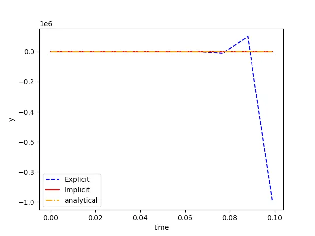
Totally diverged in Explicit time analysis

ii) dt=1.1e-3

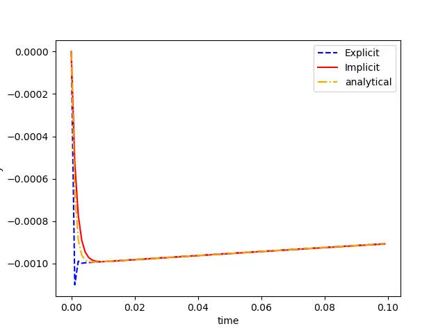
Explicit Trying to converge converged after some time analysis

iii)dt=1.8e-3

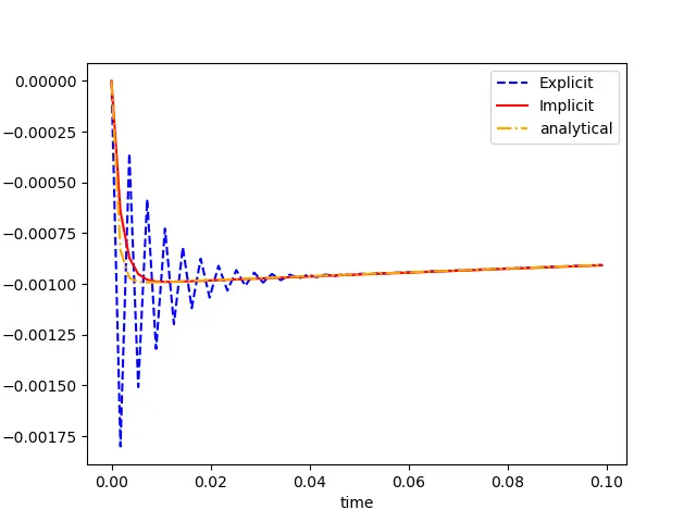
The initial time step the solution become unstable linearly after 0.04s solution started to converge

Converge

iv) dt=1e-4

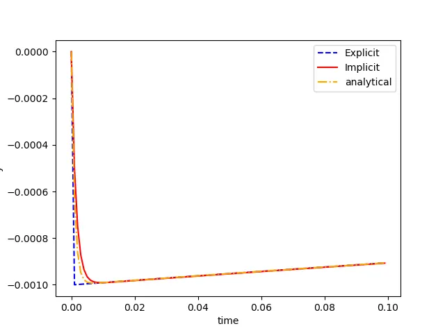
Explicit trying to converge entire solution initial & final solution is converged to an analytical solution but there is a small error or diverged in initial time step

v) dt=1.8e-4

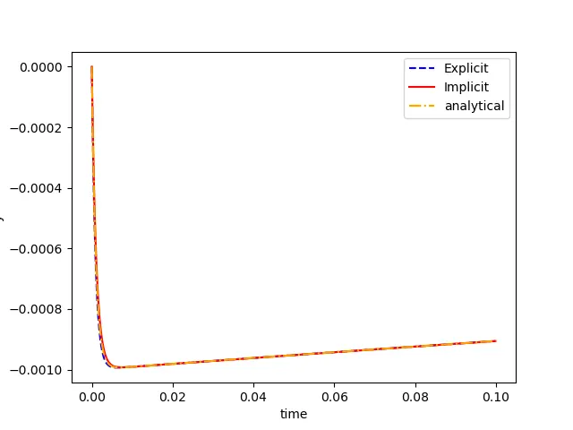
when dt=total time/ constant is < value the solution , it becomes unstable

2. How does stability affect engineering simulations

We know that an unstable solution is characterized by exponentially growing errors. These errors or residuals are a direct function of the derivatives of the quantities being solved in the solution. These residuals directly correspond to the spurious oscillations of the solution and would result in a totally unphysical solution. Such a solution is doomed to fail and cannot be used in real-time.

On the contrary, a stable solution is characterized by decreasing residuals. This means that the oscillations in the solution decrease as the solution advances and over time settle to give a steady state value. Such a solution is what is desired while performing numerical simulations.

It is important to note that a barely stable solution is not enough for engineering simulation which can be achieved by satisfying the stability condition. The solution also needs to be accurate which can be achieved by further minimizing the time step size.

explicit

a=1^e-4

when dt=total time/ constant is > a value of solution becomes unstable in an explicit analysis

dt=total time/ constant = a value of the solution becomes stable nearby value the solution start converging which is explained above

dt=total time/ constant < a value the solution becomes stable in an explicit analysis

the explicit analysis clearly shows time depended on the analysis

To make explicit analysis to stable dt=total time/ constant is = dt ( time step)

further, reduce the value of dt the solution becomes entirely stable at each time

3. Can stability condition be derived for all types of problems

Yes we can derive stability condition for all problem for example in combustion ODE is formed for a single property variable with change function of time & conflict to the numerical solution. The stability condition can only be derived for linear ODE systems.

However, for non-linear ODEs, we can predict the stability. This is done by creating a Jacobian matrix(i.e., a matrix containing the first-order derivatives of all function w.r.t. all independent variables) and computing all its eigenvalues. If all the eigenvalues are negative, it means that the solution is stable and even if one of the eigenvalues is positive, it means that the solution will be unstable. This method of predicting stability using eigenvalues of the Jacobian matrix can also be used for linear systems.