Week 5.2 - Literature review: ODE Stability

Assignment-ode stability literature review

Consider given ODE is   

dy/dx= -1000y-e^t

We know numerical scheme are two types

1.explicit

2.implicit

Euler forward difference (Explicit):

y_(n+1)=y_n+hf(y_n,t_n)

y_(n+1)=y_n+∆t(-1000y_n+e^tn)

After simplification we get

y_(n+1)=y_n (1-1000∆t)-∆te^tn

Where

(1-1000) = growth rate

If

(1-1000) <= 1 then solution is stable otherwise solution is unstable for explicit method

 Euler backward differencing for implicit method

y_n=y_(n-1)+hf(y_n,t_n)
y_n=y_(n-1)+∆t(-1000y_n-e^tn)
y_n=(y_(n-1)-∆te^tn)/((1+1000∆t))

1.when does an ODE become unstable?

If every solution  of the system close to  at initial value time t=0. In other words, is define as maximum error  that can be accommodated. This is the physical stability of ODE equation

Increments of time and space appear throughout the differential equations. Stability is achieved for explicit approach problem by limiting the value of the increment () for a particular value of space increment .if the value of  is larger than limit imposed the system becomes unstable. this is drawback of explicit method

2.How does stability affect engineering simulation?

If the value of time increment is larger than limit imposed by the stability criteria the time marching procedure become unstable. This leads to cases such as number going to infinity or it will take the square root of the negative numbers. if the value of  it will result maximum computational time. However, there is no any stability criteria for implicit method

3.can stability condition be derived for all types of problem?

We can derive stability condition for all type of problem. This is generally depending upon nature of the given function. Stability is difficult to investigate in nonlinear ODE system. The difficulty is exhibited in term of stiffness attribute. Sometimes in order to achieve stability for given ODE we make use of numerical diffusion. Numerical diffusion is a mathematical term which ensures the error in the calculation get spread out and do not add up to cause the calculation to blow up

The stability condition we use are as follows:

The Eigen value stability condition

Von Neumann stability condition

Coding approach

1.first simply this ode by using pen and paper

2.used forward differencing for explicit and backward differencing for implicit method

3.define function for explicit, implicit and for analytical solution

4.observe the results

code

"""
linear stability litrature review ODE

date=19 jan 2022

Author-siddhesh sakpal-skill lync
"""

import numpy as np

import matplotlib.pyplot as plt

import math

#time steps

dt = 1.5e-3

t_end = 0.1

def explicit_euler (t_end,dt):

	t=np.arange(0,t_end,dt)
	y=np.zeros(len(t))

	for i in range (1,len(t)):
		y[i]=y[i-1] + dt * (-1000*y[i-1]-np.exp(-t[i-1]))

	return [t,y]

def implicit_euler (t_end,dt):

	t=np.arange(0,t_end,dt)
	y=np.zeros(len(t))

	for i in range (1,len(t)):
		y[i]=(y[i-1] - np.exp(-t[i-1])*dt)/(1+1000*dt)
	return [t,y]

def analytical_solution (t_end,dt):

	t=np.arange(0,t_end,dt)
	y=np.zeros(len(t))

	for i in range (0,len(t)):
		y[i]=np.exp(-1000*t[i])*(1- np.exp(999*t[i]))/999
	return [t,y]

t,y_1 = explicit_euler (t_end,dt)
t,y_2 = implicit_euler (t_end,dt)
t,y_3 = analytical_solution (t_end,dt)


plt.plot(t,y_1,color="blue")
plt.plot(t,y_2,color="red")
plt.plot(t,y_3,color="pink")
plt.legend(["emplicit","implicit","analytical"])
plt.show()

Graphs and results

dt=1e-2

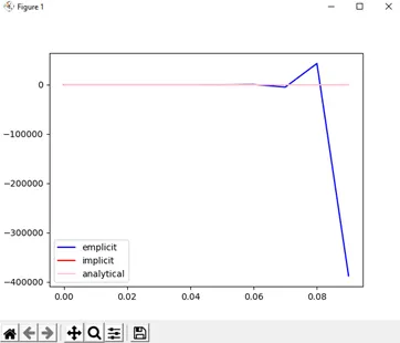
Explicit method is unstable and not converged for dt = 1e-2

dt =1e-3

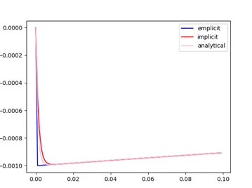
dt=1e-4

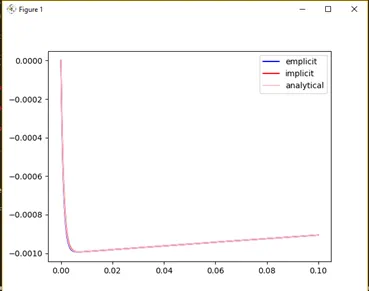
In this case solution is converged

dt=1.5e-3

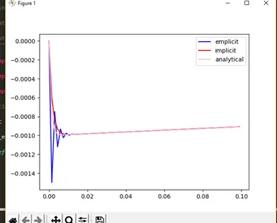
When dt =1.5e-3 solution is linearly unstable for initial time steps=0.01s after which solution is converged

Conclusion-

In this assignment we study linear stability of ODE