Week 5.2 - Literature review: ODE Stability

A LITERATURE REVIEW ON
ODE STABILITY

Aim:

To conduct a study experiment to study the stability of ODE while solving using different techniques and to answer the following questions with suitable examples:
⦁ When does a ODE become unstable?
⦁ How does stability affect engineering simulations?
⦁ Can stability condition be derived for all types of problems?

Theory:

Stability of an ODE:
According to a literature, a solution of the ODE `y ʹ = f (t, y)` is stable if for every ε > 0 there is a δ > 0 st if `y ˆ (t)` satisfies the ODE and `y ˆ (t_0 ) − y(t_0 )`≤ δ then `y ˆ (t) − y(t)` ≤ ε for all `t ≥ t_0`, i.e., rules out exponential divergence if initial value is perturbed.
For example, consider a simple ODE of the form;
`y(t) = y_0e^(lamdat)`
`y' = lamday`
If `lamda` > 0: exponential divergence : every solution is unstable,
If `lamda` < 0: every solution is asymptotically stable
If `lamda` complex:
⦁ `e^(lamdat) = e^(at) (cos(bt) + i sin(bt))`
⦁ `Re(lamda)` is a. This is oscillating component multiplied by a real amplification factor.
⦁ `Re(lamda)` > 0: All unstable; `Re(lamda)` < 0: All stable.

Effect of Stability on Engineering Simulations:
Let us consider a very simple simulation problem which involves 1D Linear convection equation. In this problem, the equation is given as, `delu/delt + c(delu/delx) = 0`
where, `delu/delt` is time derivative,
`c` is the constant convection coefficient which shows the linearity of the function,
`delu/delx` is the spatial derivative which describes the Convection term.
This simulation experiment was to compare the original and end velocity for different time-steps using Matlab Software.
Discretizing the time derivative using Forward Differencing Scheme and the convection term using Rearward Differencing Scheme,
`(u_(i)^(n+1) – u_(i)^(n))/dt = -c(u_(i)^n – u_(i-1)^n)/dx`
where, ‘n’ represents the time-step of the time marching method, in which we establish the velocity parameter at every node in one time and using these values, to evaluate the velocities in the next time-step.
‘i’ represents the node used for discretizing the convection function.
In the above discretization method, the whole RHS term is with respect to the same time-step ‘n’ and not the next time step. So, this is called as ‘Explicit Form’, since we know all the values of the RHS terms.

• The whole program for discretization of 1D linear convection equation is coded and the plots are created using Matlab Software.
• In this program, the total length of the domain ‘l’, convection coefficient constant ‘c’ and time-step ‘dt’ is defined and the function program for discretizing the equation and the value of velocities at every node in each time-step is determined and plotted, is called into the main program.

% Program for 1 Dimensional Linear Convection equation
% du/dt + c(du/dx) = 0; where, 'du/dt' is time derivative, 'c' is the
% constant convection coefficient which shows the linearity of the function,
% 'du/dx' is thespatial derivative which describes the Convection term.
clear all;
close all;
clc;

% Discretizing the equation, we get, (u(i)@(n+1)-u(i)@(n))/dt = -c(u(i)@(n)-u(i-1)@(n))/dx;
% where the time & spatial derivative uses Forward & Backward differencing scheme respectively.  
% Inputs to this function is;
l = 1;% domain length in 'm'
c = 1;% constant convection coefficient in 'm/s'
dt = [1e-4, 1e-3, 1e-2, 1e-1];% time steps 's'

% Results of the 1-D linear convection function
one_dim_linear_conv_func_2(l,c,dt);

• In the function program, the number of grid points ‘n’ for which the function is discretized, spatial location of the grid points ‘x’ and other additional inputs required for calculation of velocities at all the grid points are defined. Especially we need to give the initial conditions, i.e., the values for velocity in the 1st time step is determined to find the values in the next time-step. Also, the nodes from where the 2 m/s velocity starts to where it ends is defined by using the ‘min (abs (x- (value of grid point where it will start or end))’. So, the difference in the value where the minimum occurs is the closest point to our desired node, and that node is chosen for start and end nodes for 2 m/s velocities. For comparison of original and end velocities for different values of ‘n’, the initial velocity is saved in a separate variable. For using the initial conditions in determining the new velocity values of the next time-step, the velocities are stored in a temporary variable from which the previous values of velocities can be used.

% Function program for n grid points;
function one_dim_linear_conv_func_2(l,c,dt)
for k = 1:4
    % additional inputs for the function;
    n = 80;% grid points
    x = linspace(0,l,n);% spatial points for grid points location
    dx = l/(n-1);% since total length l = (n-1)*dx

    u(1:n) = 1;% initializing velocity temporarly to the initial value of velocity 1 m/s
    % Boundary condition;
    u(1) = 1;
    % For x = 0.1 to 0.3, (or near approximate value of 0.1 to 0.3)the value of u = 2.
    b=0.1;
    d=0.3;
    [x_start, n_start]=min(abs(x-b));% abs() command give the absolute value of the x-b,
    % min(abs(x-b)) gives the minimum value of the x and its index. 
    [x_stop, n_stop]=min(abs(x-d));% this is the default format in matlab
    u(n_start:n_stop) = 2;% so at these nodes, the value of u is 2m/s.

    tend = 0.4;
    t = (0:dt(k):tend);% total time step span
    figure(2);
    hold on;
    plot(t,dt(k),'*','color',[rand rand rand]);
    xlabel('Simulation time, T');
    ylabel('Time-step, dt');
    title('Plot for Simulation Time vs Time-Step');
    hold off;
    uinitial = u;% initial values of u for plot
    uold = u;% temporary saving of u for iteration continuation
    for j=1:length(t) % length(t) is no. of time steps
        for i=2:n
            % Using 1st order forward differencing for time derivative and
            % 1st order backward differencing for space term
            u(i) = uold(i) - (c*dt(k)/dx)*(uold(i) - uold(i-1));
        end
        uold = u;% to update previous velocities for next time step

        figure(1);
        txt = ['End Velocity at ' num2str(dt(k)) ' dt'];
        subplot(3,2,[1,2]);
        plot(x,uinitial);
        xlabel('Values of x');
        ylabel('Initial velocity');
        title('Comparing Velocities in 1-D linear Convection at different Time-steps');
        axis([0 1 0 2]);
        subplot(3,2,k+2);
        plot(x,u,'color','r');
        xlabel('Values of x');
        ylabel(txt);
        axis([0 1 0 2]);
        pause(1e-3000)
    end
end
end

• The 1st ‘for’ loop is used for the time step variation and the 2nd ‘for’ loop is for the different time-step values for the same number of nodes. We track all the time-steps in a single plot window to create a simulation of how the velocity graph moves with respect to time. Also to compare the original and final velocity for different values of ‘n’ in a single figure window is done using the ‘subplot()’ command to split the plot into 3 halves, where the initial velocity is at the top and the 4 end velocities for the 4 values of ‘dt’ is at the middle and bottom of the plot.

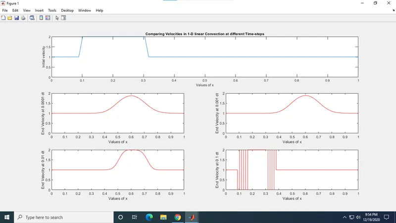
In the above plot, we can observe that the velocity reduces as it moves with each time-step and finally a lower value of velocity is obtained. This means that the velocity diffuses with time but this is not possible because we do not have any diffusion terms in the equation. So, how this diffusion occurs is because we took the 1st order differencing scheme where ignores the higher order terms starting from 2nd order. These ignored terms sum up together as an error term known as the truncation error. This error acts as the 2nd order diffusion term which is called as the artificial or numerical diffusion, which is responsible for the drop in velocity values. These plot values correspond to the Courant Number ‘C’ which is the necessary condition for convergence in any ODE or PDE involving explicit form.

Also, in the above plots, we can see that the value of the peak at the end of each simulation time, t, increases (i.e., diffusion decreases) with corresponding increase in the value of time-step, i.e., from `‘1e^-4’` to `‘1e^-1’` for a constant number of nodes, but suddenly becomes unstable at the 4th plot `‘dt = 1e^-1’.` This is because of the CFL criteria also known as the CFL condition which is given by ‘C = udx/dt <=Cmax’. This criterion shows that the Courant Number increases with increase in time-step ‘dt’ for constant ‘dx’, but still, it must be within the maximum Courant Number ‘Cmax’ which is usually ‘1’ for Explicit Time Marching technique. So, in the case where `‘dt = 1e^-1’,` the Courant Number exceeds the value of ‘1’ for that particular dx value. Thus, in order to stabilize the results with higher accuracy, we need to increase the number of nodes or decrease ‘dt’ both only upto a stable limit, that is where the Courant Number is lesser than or equal to 1. The CFL condition explains that the distance that any information travels during the timestep length (dt) within the mesh must be lower than the distance between mesh elements (dx).

Can stability condition be derived for all types of problems:
The stability condition can be easily derived for linear ODE systems. However, for non-linear ODEs, we can predict the stability but still it depends upon a lot of criteria based on the complexity of the problem we undertake. One method is by determining a Jacobian matrix, i.e., a matrix containing the first-order derivatives of all function w.r.t. all independent variables, and computing all its eigenvalues. If all the eigenvalues are negative, it means that the solution is stable and even if one of the eigenvalues is positive, it means that the solution will be unstable. As discussed, in the previous question, which involves CFL number in predicting the stability, we can provide a very stable result if the CFL < 0.7. But still, if we are able to reduce it too much, the solution will be stable but the results will have a poor accuracy when compared with it's Analytical results, which is again based on the type of problem that is undertaken for study.

Results:

Thus, the study experiment to study the stability of ODE while solving using different techniques and to answer the questions was conducted successfully.