Week 5.2 - Literature review: ODE Stability

Aim: - To perform a study on Ordinary Differential Equation solution stability o Euler's Method.

Objective: -

1. To write a program in python for Explicit and implicit method for Euler method and compare results for following ODE -

`dy/dt = -1000y-exp(-t)`

1. To discuss the stability criterion for ODE solution based on above result.

Theory: -

Ordinary Differential Equation(ODE) -

It is an equation which consists of one or more functions of one independent variable along with their derivatives. A differential equation is an equation that contains a function with one or more derivatives. But in the case ODE, the word ordinary is used for derivative of the functions for the single independent variable.

In other words, the ODE is represented as the relation having one independent variable x or t, the real dependent variable y, with some of its derivatives.

Its examples are newton second law of motion, radioactive decay etc.

`m*(d^2 y)/(dt^2 ) = f(y),`

Euler's Method -

It is a first-order numerical procedure for solving ordinary differential equations (ODEs) with a given initial value.

Explicit – It the first order differencing scheme which calculate the state of a system at a later time from the state of the system at the current time.

Implicit – It is a first order backward Differencing scheme which calculate solution by solving an equation involving both the current state of the system and the later one.

Considering the general form of ODE:

`dy/dt = -1000*y-e^(-t), y(0)=0`

Explicit formulation –

`(y^(n ew) -y^(old))/dt = -1000*y^(old) - e^(-t)`

`y^(n ew)= y^(old) +dt*(-1000*y^(old)-e^(-t))`

Implicit formulation –

`(y^(n ew) -y^(old))/dt = -1000*y^(n ew) -e^(-t)`

`y^(n ew)= (y^(old)-e^(-t)*dt)/(1+1000*dt)`

Analytical solution –

`y= (e^(-1000*t)*(1-e^(999*t)))/999`

Stability - Numerical algorithms can damp or magnify the fluctuation (error) in solving the differential equation. The algorithm which damp the error to an acceptable margin and provide a stable solution.

Code: -

"""
program to understand stability of ODE "dy/dt = -1000y-exp(-t)"

"""

import numpy as np
import matplotlib.pyplot as plt

# defining explicit function
def explicit_euler(t_end,dt):
	t = np.arange(0,t_end,dt)
	y = np.zeros(len(t))

	for i in range(1,len(t)):
		y[i] = y[i-1] + dt*(-1000*y[i-1] - np.exp(-t[i-1]))
	return [t,y]
# defining Implicit function
def implicit_euler(t_end,dt):
	t = np.arange(0,t_end,dt)
	y = np.zeros(len(t))

	for i in range(1,len(t)):
		y[i]= (y[i-1] - np.exp(-t[i-1])*dt)/(1+1000*dt)
	return [t,y]
# defining exact analytical function
def anytcl_value(t_end,dt):
	t = np.arange(0,t_end,dt)
	y = np.zeros(len(t))

	for i in range(1,len(t)):
		y[i]= (np.exp(-1000*t[i])*(1-np.exp(999*t[i])))/999
	return [t,y]
# Assigning values for end time an time step
t_end = 0.1
dt = np.linspace(1e-3,2e-3,6)

# Apply loop to call and evaluate the above defined function for range of time step
for j in range(0,len(dt)):
	[t,explicit] = explicit_euler(t_end,dt[j])
	[t,implicit] = implicit_euler(t_end,dt[j])
	[t,analytical] = anytcl_value(t_end,dt[j])
        
        # plotting calculated values
	plt.figure(j+1)
	plt.plot(t,explicit,'--',color='red')
	plt.plot(t,implicit,'--',color='blue')
	plt.plot(t,analytical,'--',color='green')
	plt.xlabel('time')
	plt.ylabel('y')
	plt.legend(['Explicit','Implicit','analytical'])
	plt.title('Function value at time step = %f sec' %dt[j])

plt.show()

Results: -

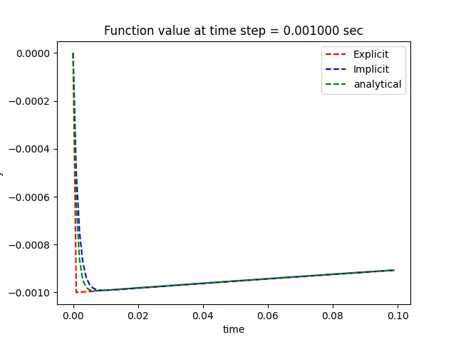
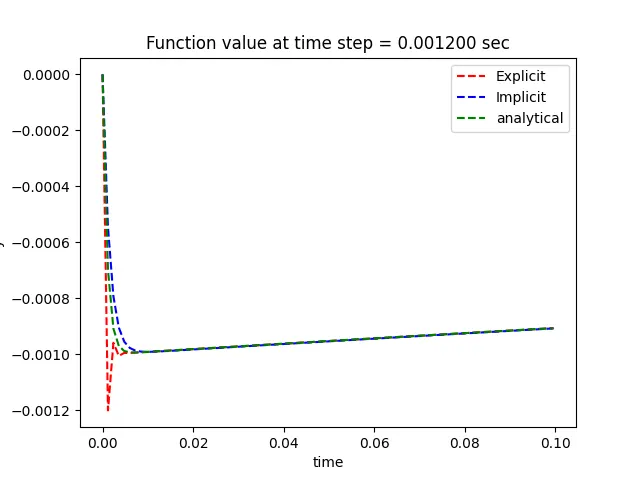
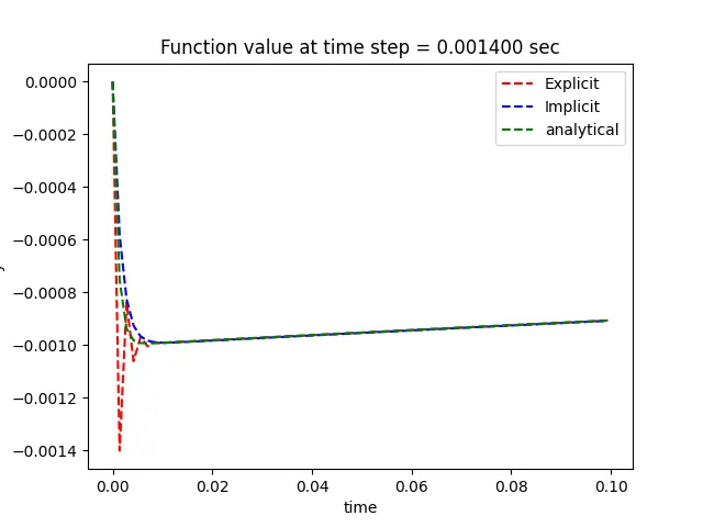
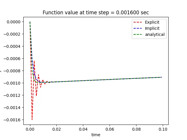
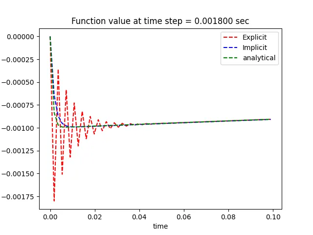
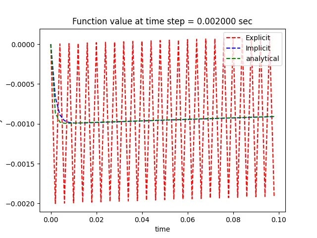
Conclusion: -

• Expicit method tend to become Unstable after a certain time step whereas, implicit method remains more accurate and closely imitates the exact solution of the function.
• For explicit stablity - As first order differencing scheme is error proportional to square of time step and after certain time step this becomes perodic/harmonic and give wrong results.

the criteria or stable results or Euler's expicit method

`abs(1-lambdah) < 1` `=> h < 2/lambda`

here h is time step which is dt and `lambda` is coefficient of `y^(old)*dt` = 1000

`y^(n ew)= y^(old) (1-1000*dt)- e^(-t)*dt`

hence the value shoot off near 2e-3 in the above plots.

• For implicit stability - the criteria for implicit method

`abs(1/(1+lambdah)) <1 => h>0`

hence the impicit stay in proper limit for all time step and provide better results at the expance of coputtion time.

• Stability play a major role in the engineering simulation. An unstable result can give wrong/meaning less results. Therefore stable numerical schemes are employed for better accuracy and simulation. Cfl criterial is already employed for explicit schemes in convection simulations which is to limit cfl less than 1.
• Yes stability can be defined for all type o system, but impicit scheme does not require one as it produce more ccurate values, but for explicit systems on should be in limits for stability.