Week 5.2 - Literature review: ODE Stability

LITERATURE REVIEW: ODE STABILITY

AIM: A literature review is a great way to assimilate a large amount of data and convert it to a form that you can understand.

OBJECTIVE:

• A literature review is a great way to assimilate a large amount of data and convert it to a form that you can understand
• When does an ODE become unstable?
• How does stability affect engineering simulations?
• Can stability conditions be derived for all types of problems?

CODE AND SOLUTIONS

When does an ODE become unstable?

If every solution `psi(t)` of the system close to `phi(t)` at initial time t = 0 remains close for all the future times. In other words, the stability definition talks about the maximum error `abs(psi(t) - pgi(t))` that can be accommodated. This is the physical stability of an ODE equation.

When the same equation is solved numerically, 'Numerical Stability comes into play. The step size chosen to solve the equation numerically plays an important role in numerical solvers.

How does stability affect engineering simulations?

With various time step (dt) variation of result which is shown in the graph for the explicit method is time various method implicit is a time-independent problem. A constant solution called equilibrium. An equilibrium solution called Stability is an important condition to conflict the function of the variant to the numerical solution to the analytical result. when the function approach close to it for further all time. If a function does not remain constant to time when an increase then it's unstable

Can stability conditions be derived for all types of problems?

For ODE systems, stability analysis is divided into the following:

• Linear ODE Stability
• Stability of autonomous ODE systems
• Non-Linear stability systems.
• ODE stability for Multivariable systems

CODE:

import math
import matplotlib.pyplot as plt
import numpy as np


def explicit_euler(T,dt):
	t = np.arange(0,T,dt)
	y = np.zeros(len(t))
	

	for i in range(1,len(t)):
		y[i] = y[i - 1] + dt*( -1000*y[i - 1] - np.exp(-t[i - 1]))
	return [t,y]

def implicit_euler(T,dt):
	t = np.arange(0,T,dt)
	y = np.zeros(len(t))

	for i in range(1,len(t)):
		y[i] = (y[i - 1] - np.exp( -t[i - 1])*dt)/(1 + 1000*dt)

	return [t,y]

# analytical anaylsis 
def analytical_euler(T,dt):
	t = np.arange(0,T,dt)
	y = np.zeros(len(t))

	for i in range(1,len(t)):
		y[i] = (np.exp( -1000*t[i])*(1 - np.exp((1000 - 1)*t[i])))/(1000 - 1)

	return [t,y]


T = 0.1
dt = 1.5e-3

t,y_explicit = explicit_euler(T,dt)
t,y_implicit = implicit_euler(T,dt)
t,y_analytical = analytical_euler(T,dt)
plt.plot(t,y_explicit,'--',color='green')
plt.plot(t,y_implicit,'-.',color='blue')
plt.plot(t,y_analytical,color='red')
plt.xlabel('time')
plt.ylabel('y')
plt.legend(['Explicit','Implicit','analytical'])
plt.savefig('euler_time_analysis_c2')
plt.show()

GRAPHS

dt = 1e - 2

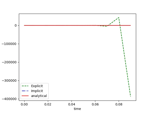
We see in the above graph when dt = 1e-2 there is a Total divergence in Explicit time analysis

dt = 1e - 3

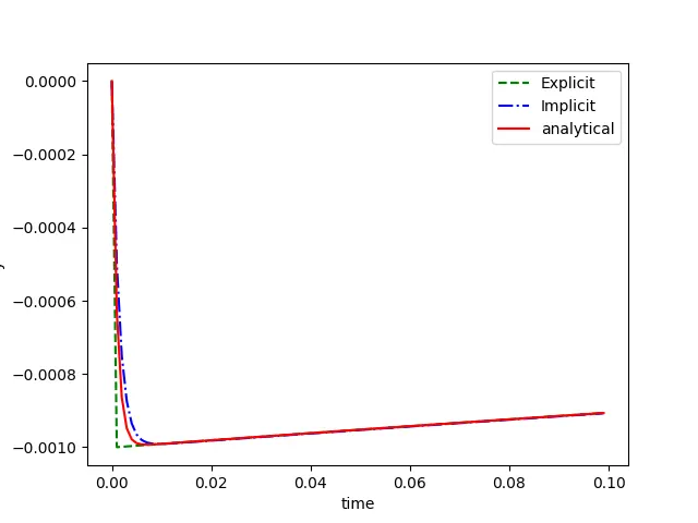
We see in the above graph when dt = 1e-3 In the explicit scheme are getting converged when compared to the previous plot.

dt = 1e-4

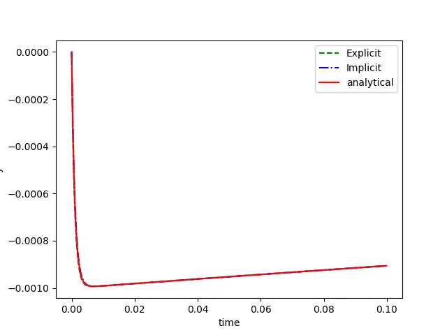
When dt = 1e-4 the explicit analysis is fully converged with an analytical solution when the solution satisfies dt=total time/ constant is greater.

dt = 1.5e-3

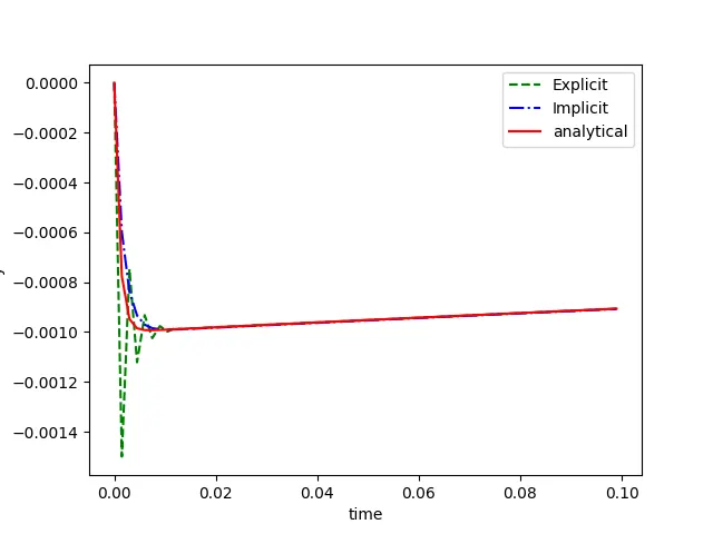
When dt = 1.5e-3 the solution becomes linearly unstable for the initial time step 0.01s, after which the solution started to converge.

Conclusion

ODE is important for all applications not only restricted to engineering solutions.

For explicit analysis, the value of dt (change in time) is analyzed with a time step