Week 5.1 - Non-Conformal Meshing and Solving a Cold plate model

Aim:

To perform the Non-Conformal Meshing on a Cold plate model

Objective:

To perform the analysis for a two-heated plates model, cooled by water circulating inside the cold-plate cavity, as well as by air driven by natural convection externally. And separately meshed assemblies will be employed to reduce the overall mesh count in the domain.

The following objects are created in the model as per the given design specifications:

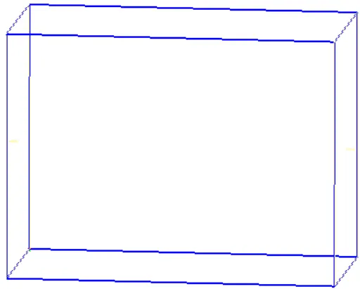
Cabinet: It is the bounding box within which the governing equations are solved.

Geometry:

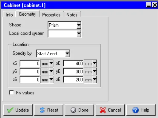
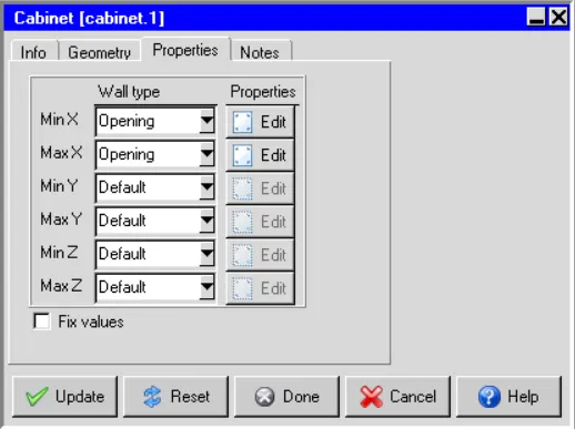
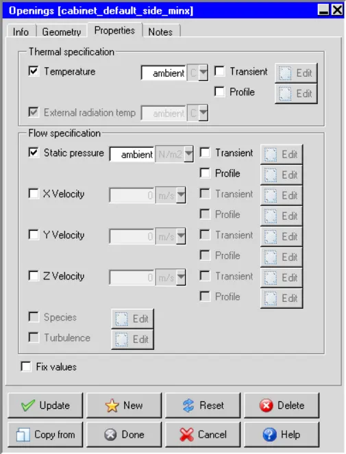
The Default wall type defines the specified Cabinet wall to have no thickness and have zero velocity and zero heat flux (adiabatic) boundary conditions. The Opening wall type defines the specified Cabinet wall as an opening object.

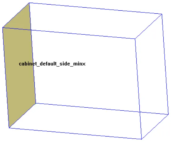
cabinet_default_side_minx

cabinet_default_side_maxx:

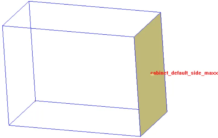
The following properties are attributed to cabinet_default_side_maxx:

Static pressure: ambient (Gauge Pressure: 0 N/m2)

Solid_block: It is located between the two heated plates, and forms the cavity within which cooling water is circulated

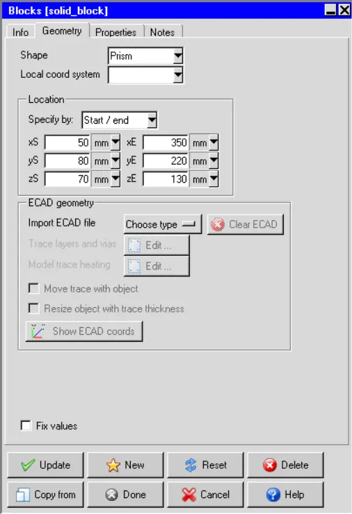
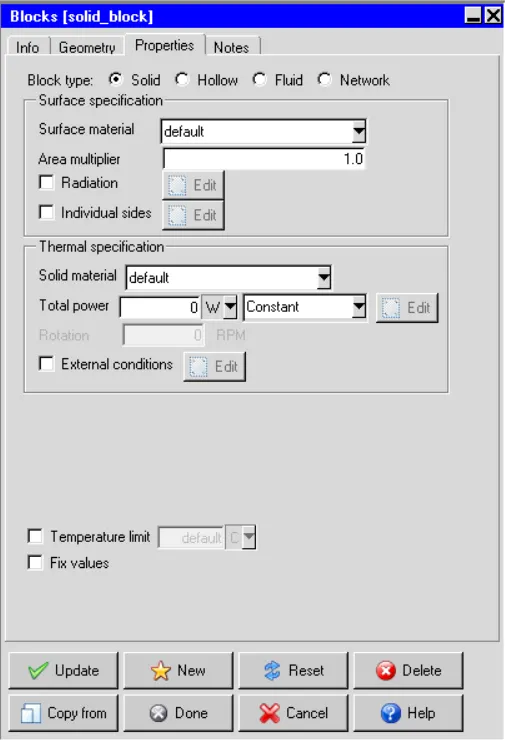
The image attached below shows the geometry with Solid_block highlighted.

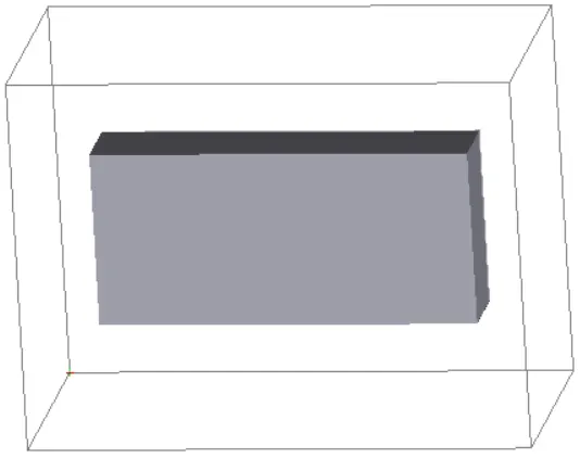
Solid_block is a solid object with no available cavity for the circulating fluid. In order to simulate the fluid cavity, a fluid block of appropriate dimensions is defined with a higher meshing priority than the Solid_block.

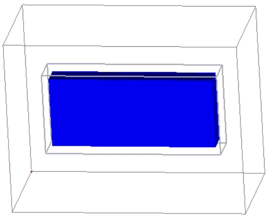
Fluid_block: It forms the fluid domain, which represents the circulating fluid, inside Solid_block. It is imparted a higher meshing priority than the Solid_block.

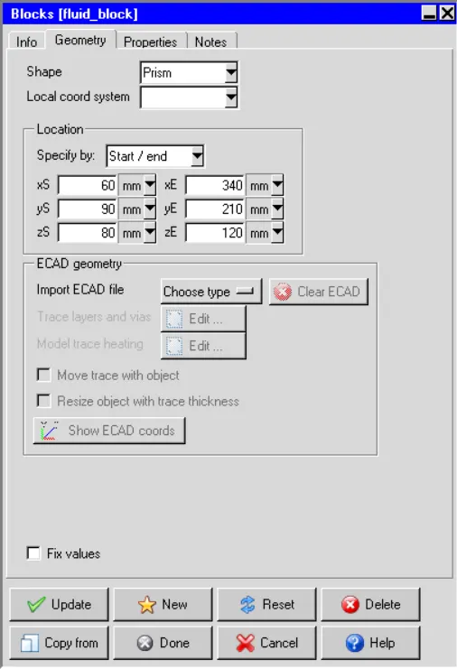
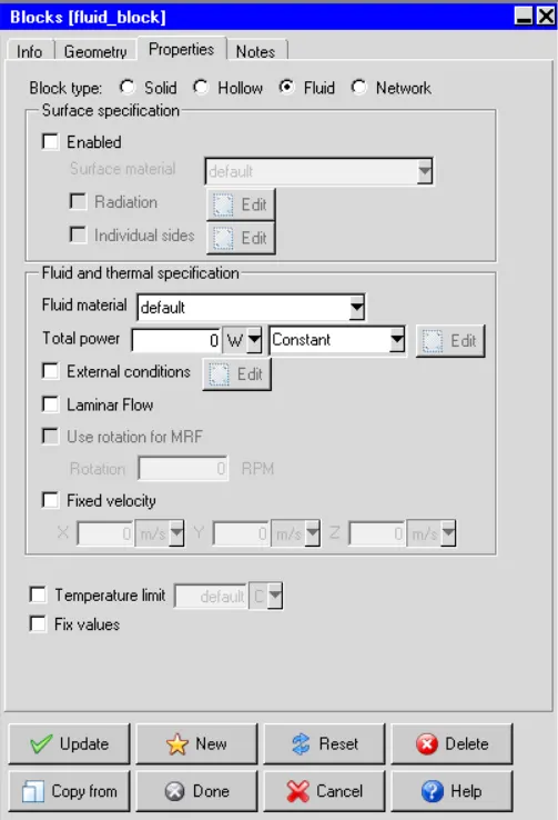
The image attached below shows the geometry with Fluid_block highlighted.(Fluid_block is inside the Solid_block)

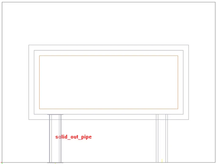
Solid_out_pipe: It carries the circulating fluid leaving the cold-plate cavity.

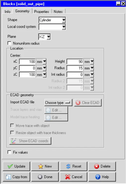
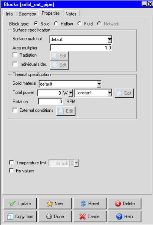
The image attached below shows the geometry with Solid_out_pipe highlighted. We can see hollow pipe with 5mm thickness connected to the fluid block

Solid_in_pipe: It carries the circulating fluid entering the cold-plate cavity

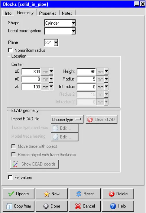
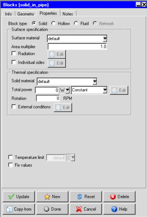
The image attached below shows the geometry with Solid_in_pipe highlighted. We can see a hollow pipe with a 5mm thickness connected to the fluid block

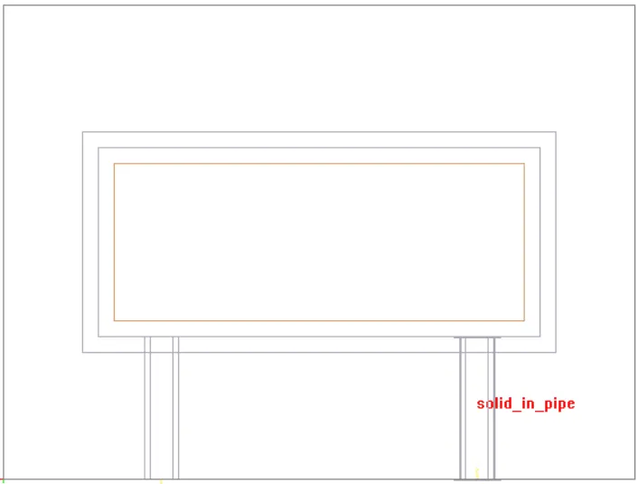
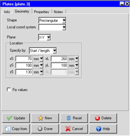
Plate_2: It forms one of the heated plates which is being cooled by the circulating fluid (inside the cold-plate cavity) on one side and by an air driven by natural convection on the other side.

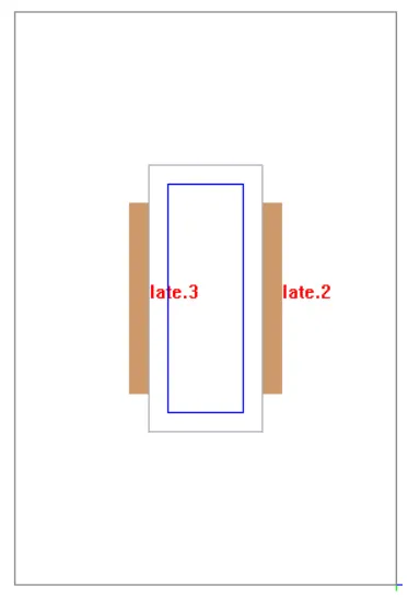
Here plates are created on both sides of the solid block

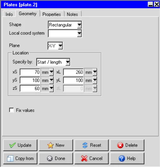
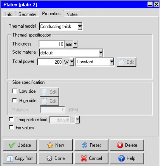
we can see the plates in the figure below

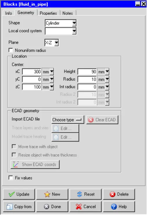
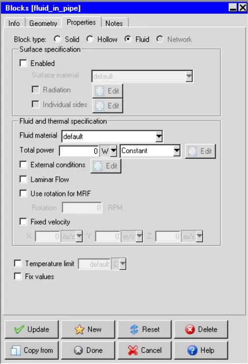
Fluid_in_pipe:

It forms the fluid domain, which represents the circulating fluid, inside Fluid_in_pipe.

Fluid_out_pipe:

It forms the fluid domain, which represents the circulating fluid, inside Fluid_Out_pipe.

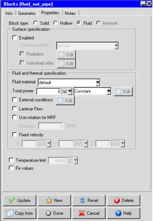
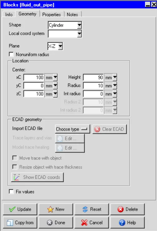
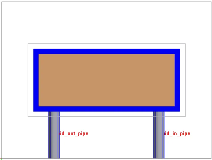
The image attached below shows the Fluid_in and Fluid_out inside the hollow pipe

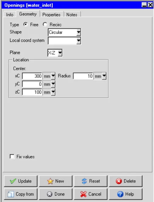
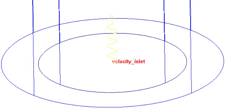
Velocity_inlet/water_inlet: It is created as an Opening object on the Min Y Cabinet wall to allow the circulating fluid to enter the Cabinet.

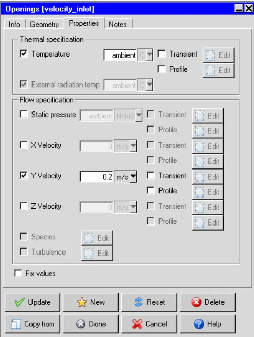
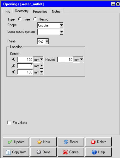
Velocity_Outlet/water_outlet:

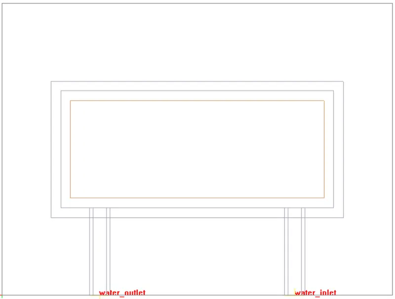
The image attached below shows the geometry with Velocity_inlet and velocity_Outlet highlighted.

Meshing:

The non-conformal mesh prevents mesh bleeding and hence yields a lower mesh count than conformal mesh while maintaining the same level of accuracy and resolution. In order to generate a non-conformal mesh, an assembly is created with the following objects:

1. Solid_block

2. Fluid_block

3. Solid_in_pipe

4. Solid_out_pipe

5. Plate_1

6. Plate_2

7. Velocity_Inlet

8. Velocity_Outlet

9. Fluid_in_pipe

10.Fluid_out_pipe

The following settings are applied to further define the assembly and after creating and defining the assembly, the following settings are applied in the "Mesh control" window:

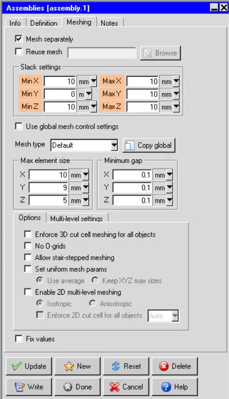
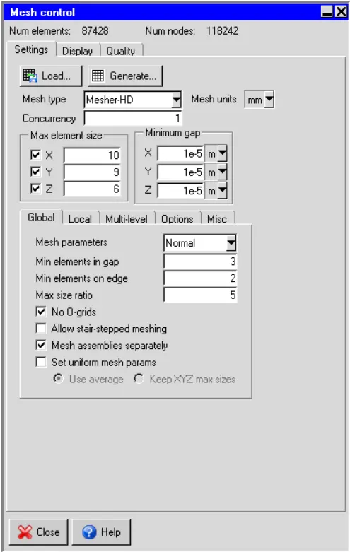
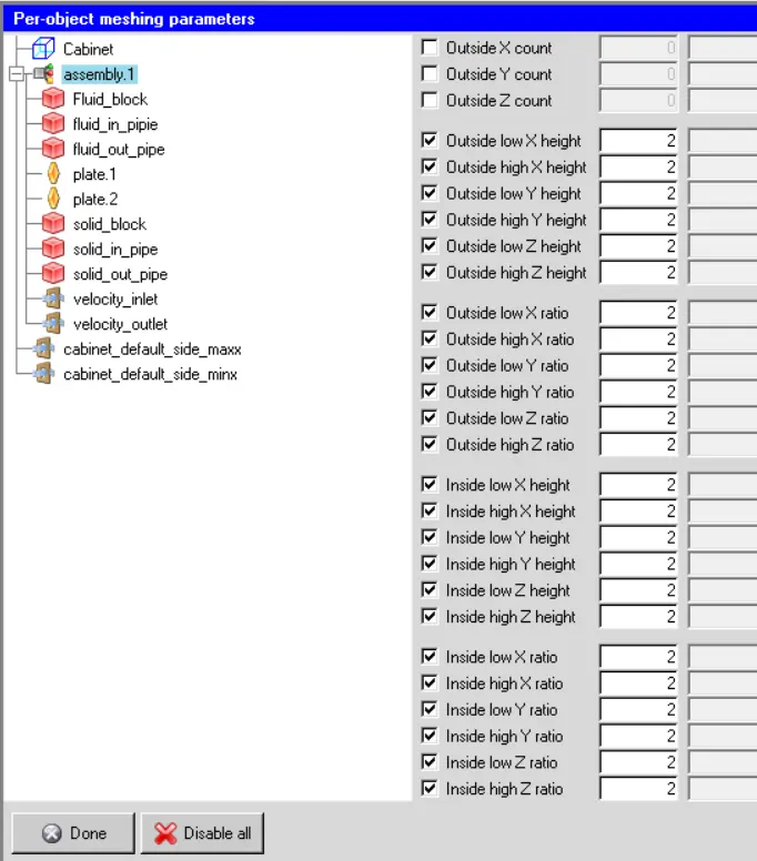
The non-conformal mesh generated using the settings outlined above contains 33964 elements and 37806 nodes. The images attached below show the mesh along different cut-planes.

1. Mesh along Z plane through the center

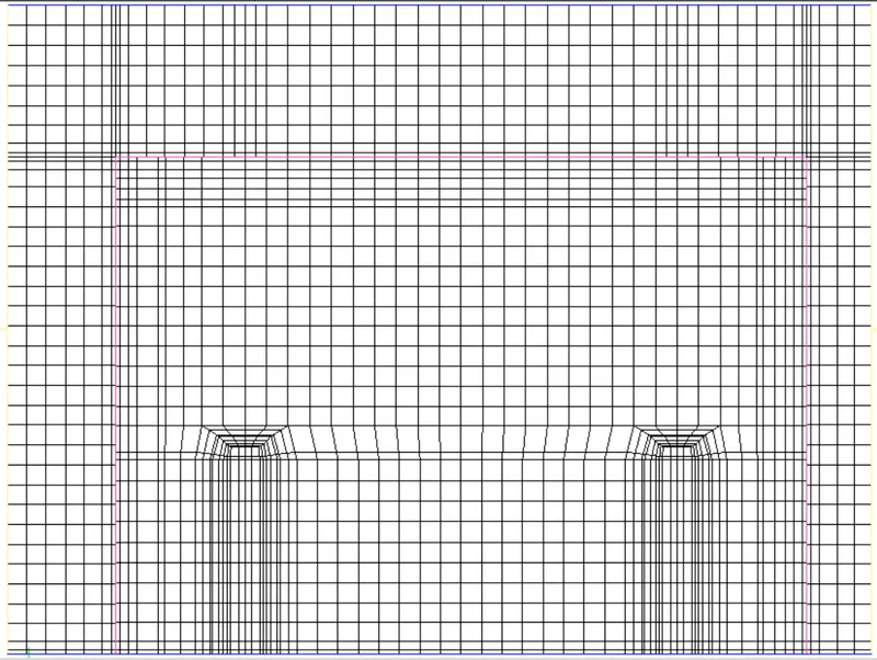
2. Mesh along Y plane through the center

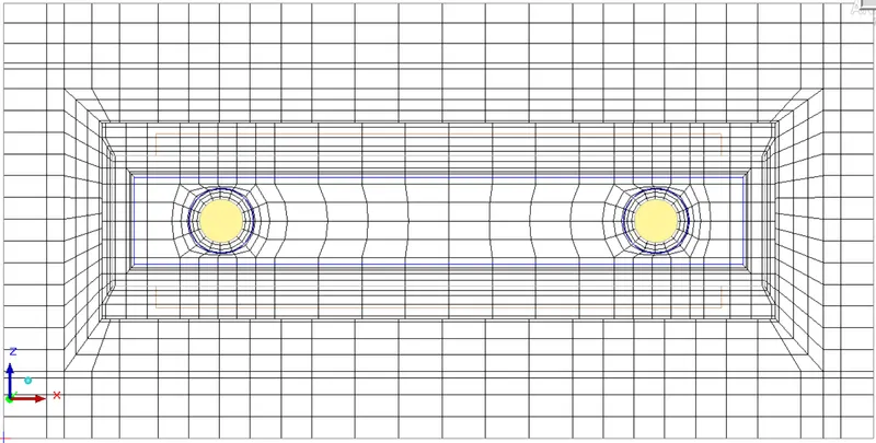
3. Mesh along Z plane through the center

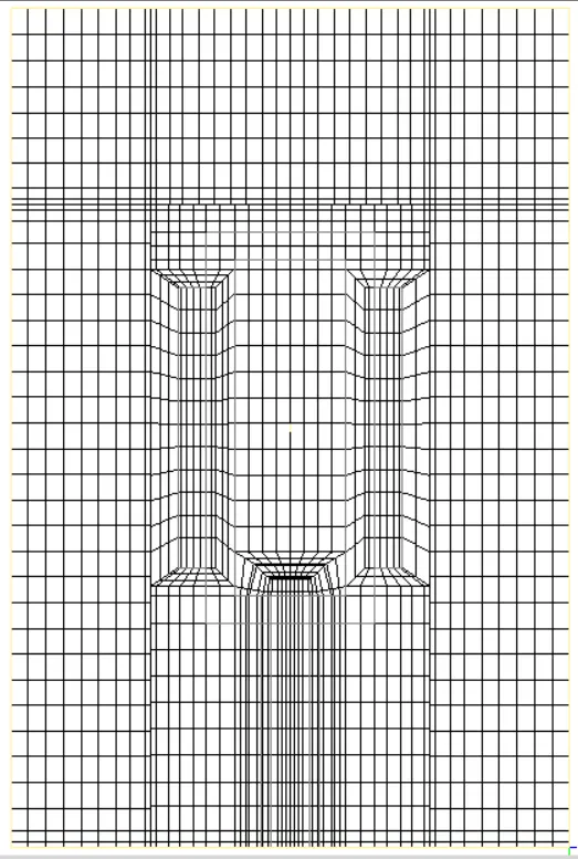
Visually, the mesh appears to be dense within and near the assembly (which is desired). The following checks are performed to further assess the mesh quality:

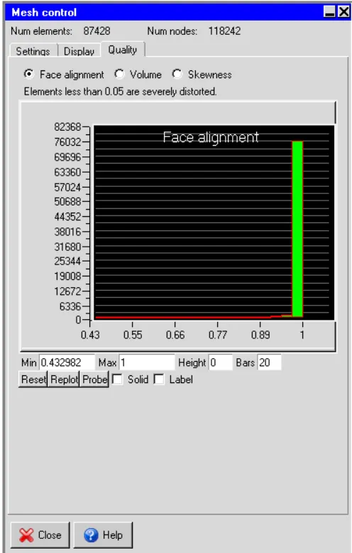
Face alignment: It is a measure of the relative face alignment between two adjacent elements in the mesh. The image attached below shows the face alignment histogram for different elements in thecurrent mesh.

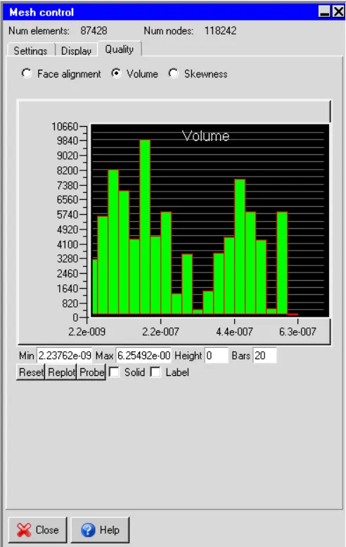
Volume: It measures the volume of all the elements in the mesh. The image attached below shows the volume histogram for different elements in the current mesh.

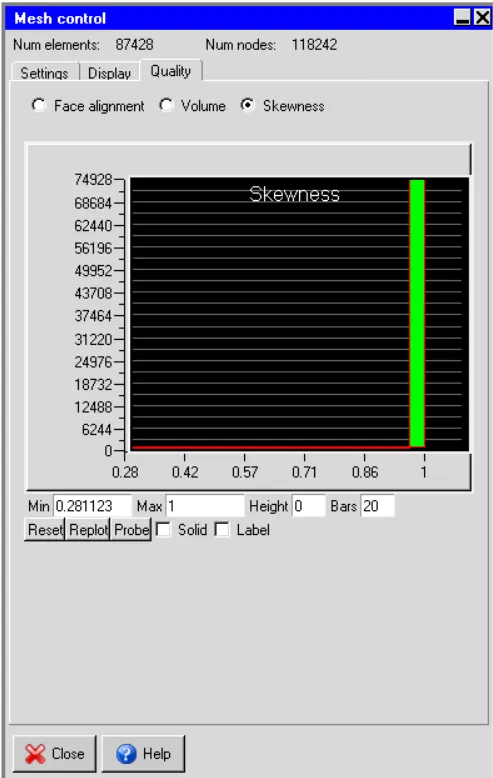
Skewness: It is a measure of how close to the ideal (equilateral/equiangular) a mesh element is. The image attached below shows the skewness histogram for different elements in the current mesh.

Solver:

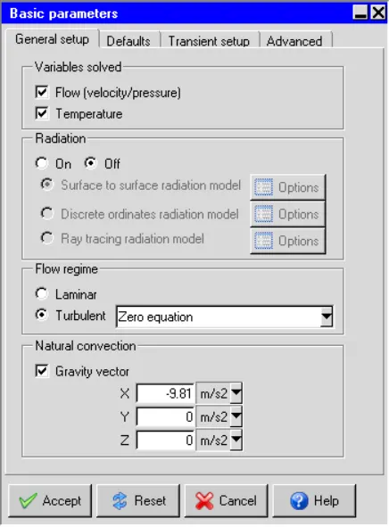
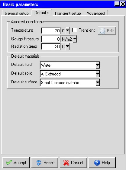
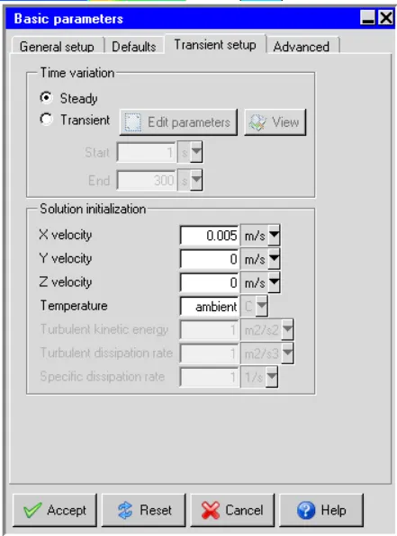
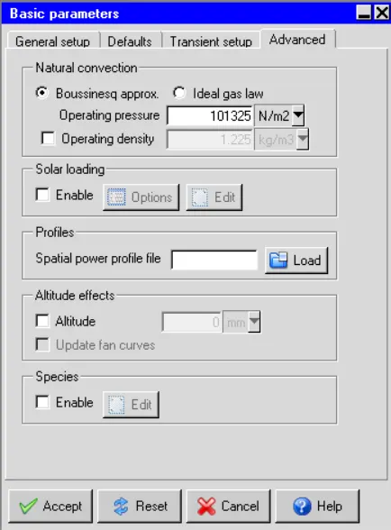
ANSYS Icepak package employs the Fluent solver engine to solve the discretized governing equations within the computational domain. The following settings are applied in the Problem setup and Solution settings nodes of the Model manager window:

Solution settings:

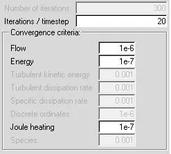
Basic settings

The image attached below shows the various parameters specified in the Basic settings node available within the Solution settings node in the Model manager window.

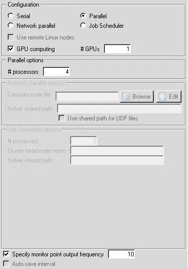
Parallel settings

The image attached below shows the various parameters specified in the Parallel settings node available within the Solution settings node in the Model manager window.

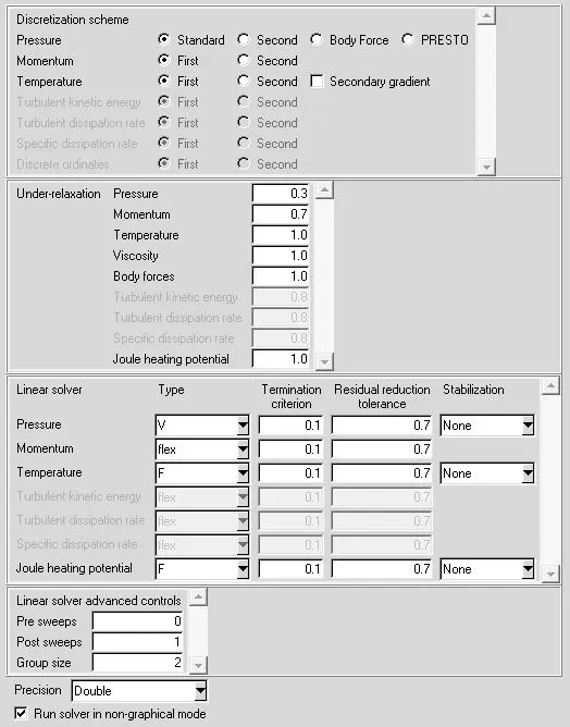
Advanced settings

The image attached below shows the various parameters specified in the Advanced settings node available within the Solution settings node in the Model manager window.

Results:

In the current section the simulation results are discussed:

Residuals

The residuals for the following governing equations are monitored:

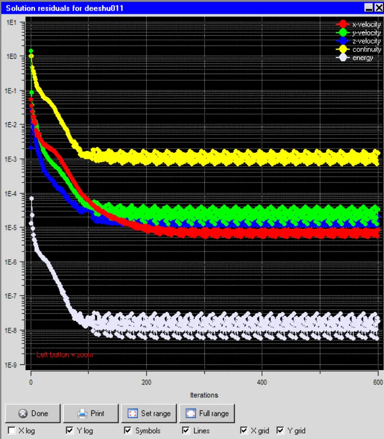
As evident from the plot, all the monitored residuals are quite small in magnitude and don't change appreciably between 200 to 600 iterations indicating that a steady state has been achieved.

Temperature monitor plots:

The following four surface probes are set up to monitor the average temperature over the specified surfaces for the entire duration of the simulation (t=0 s to t=300 s):

i. Air_in: It is used to monitor the average temperature over the object cabinet_default_side_minx.

ii. Air_out: It is used to monitor the average temperature over the object cabinet_default_side_maxx.

iii. Water_in: It is used to monitor the average temperature over the object Inlet.

iv. Water_out: It is used to monitor the average temperature over the object Outlet.

The image attached below shows the output of all four surface probes,

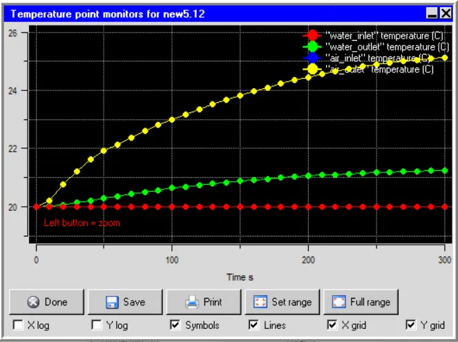
. The steady-state average temperature values measured by the four surface probes are as follows:

i. Air_in: 20 deg. C

ii. Air_out: 25.21 deg. C

iii. Water_in: 20 deg.C

iv. Water_out: 21.33 deg. C

Temperature contours

The temperature contours are plotted along different cut-planes as well as object faces to observe the temperature distribution throughout the domain at steady state

Temperature contours plotted on the Z plane through the center

The image attached below shows the steady state temperature contours plotted on the cut-plane passing through the center of the cabinet and perpendicular to the Z-axis.

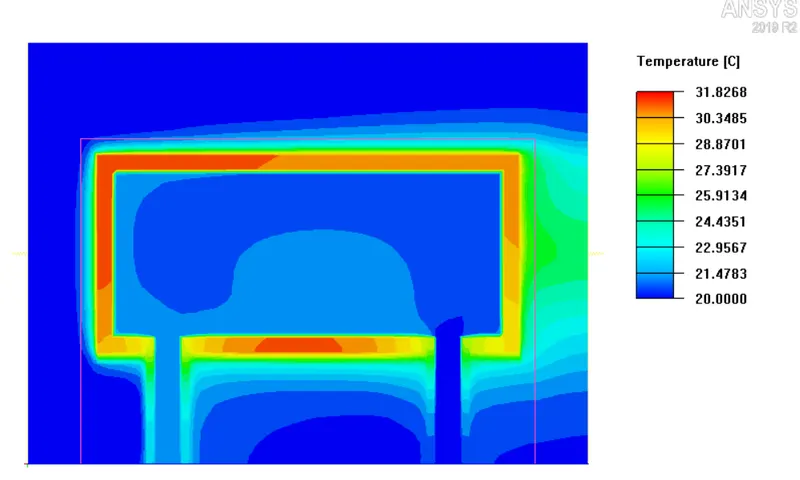
The plot clearly shows that water enters into the cold-plate cavity at ambient temperature (20 deg. C) and as it moves further inside the cavity its temperature increases. This is because of the heat transfer from Solid_block to water. The contours show the presence of thermal boundary layers around Solid_block. This is due to the heat transfer between Solid_block and air by natural convection. The thermal boundary layers on all the surfaces of Solid_block aligned along the X-coordinate grow in the +X direction since the gravitational field is directed along the -X direction.

Temperature contours plotted on the Y plane through the center

The image attached below shows the steady-state temperature contours plotted on the cut-plane passing through the center of the cabinet and perpendicular to the Y-axis.

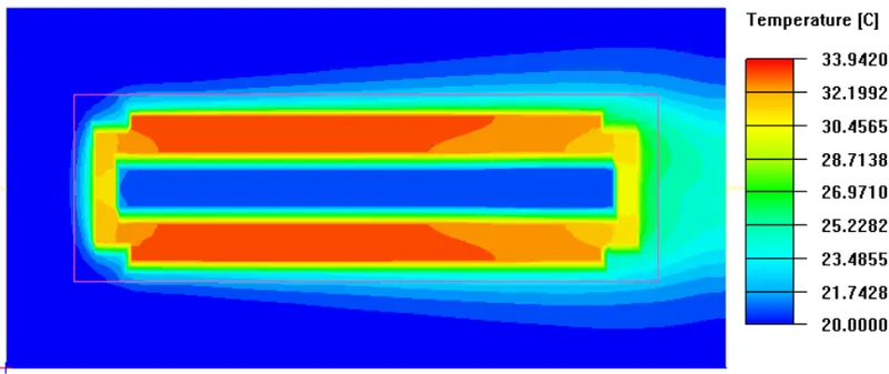
The plot shows that the heated plates achieve the highest temperature and as we move from the heated plates to Solid_block the temperature decreases. In other words, temperature gradients are present in the solid domain between the heated plates and Solid_block, with the heated plates at a higher temperature. This indicates that the heated plates lose heat to Solid_block. Similarly, temperature gradients are also present as we move from Solid_block to Fluid_block, with Solid_block at a higher temperature. This indicates that Solid_block loses heat to Fluid_block. Hence the heat generated in the heated plates is transferred to Solid_block (by conduction) from where it is finally dissipated into Fluid_block (by forced convection). The contours also clearly show the presence of thermal boundary layers on the outer surfaces of the heated plates. These thermal boundary layers are formed as a result of the heat transfer between the heated plates and the ambient air (by natural convection), and they (thermal boundary layers) grow against the gravitational field.

Fluid face temperature contours:

The image attached below shows the steady-state temperature contours plotted on the outer faces of all the objects in the geometry that are defined as a fluid type.

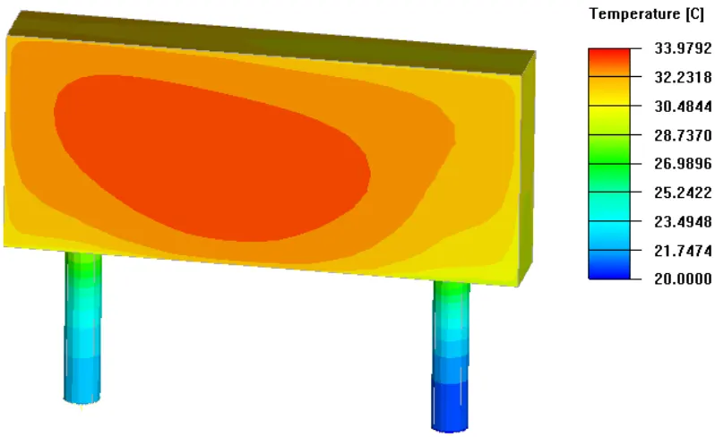
According to the contour plot the maximum temperature (33.979 deg. C) is observed beneath the heated plates. The outgoing fluid is hotter than the incoming fluid which indicates that the circulating fluid gains heat as it moves through the cold-plate cavity.

Solid face temperature contours

The image attached below shows the steady-state temperature contours plotted on the outer faces of all the objects in the geometry that are defined as a solid type.

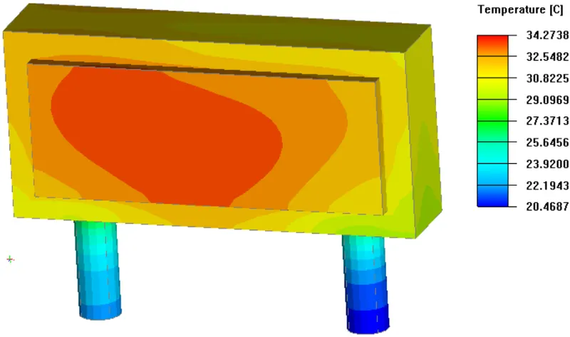
According to the contour plot, the maximum temperature (34.2738 deg. C) is observed over the heated plates.

Velocity contours:

The velocity contours are plotted along different cut planes to observe the velocity distribution throughout the domain at a steady state.

Velocity contours plotted on the Z plane through the center

The image attached below shows the steady state velocity contours plotted on the cut-plane passing through the center of the cabinet and perpendicular to Z-axis.

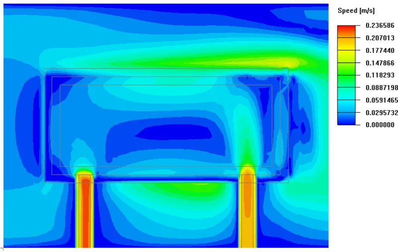
The contour plot clearly shows the convection cells in the XY plane present around Solid_block at Min Y and Max Y walls. These convection cells represent the convection currents established in the ambient air due to the heat transfer between Solid_block and ambient air by natural convection.

Velocity vectors:

The velocity vectors are plotted along different cut-planes to gain further insight into the velocity distribution throughout the domain at steady state

Velocity vectors plotted on the Z plane through the center

The image attached below shows the steady state velocity vectors plotted on the cut-plane passing through the center of the cabinet and perpendicular to Z-axis.

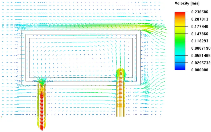
The vector plot clearly shows the flow directions of incoming fluid, outgoing fluid and air but is unable to capture the convection cells observed in the velocity contour plot.

Velocity vectors plotted on the Y plane through the center

The image attached below shows the velocity vectors plotted on the cut-plane passing through the center of the cabinet and perpendicular to T-axis.

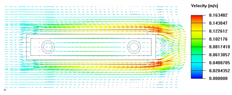
The vector plot shows that air accelerates as it moves up against gravity due to natural convection. The vector plot successfully captures the recirculation zone behind Solid_block but is unable to capture the convection cells observed in the velocity contour plot.

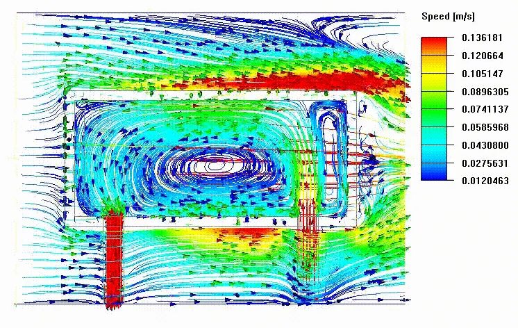
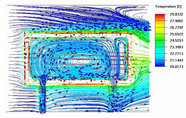
Animation is shown below:

Conclusion:

In the current project, CFD simulation of the cold-plate cavity was performed using ANSYS Icepak. The model was created using the given design specifications. Non-conformal meshing was employed with local mesh refinement using object parameters. A zero equation turbulence model was employed to capture turbulence. The gravity vector was defined along the -X direction. Four surface probes were defined to monitor the average temperature over four surfaces in the computational domain. The discretized governing equations were solved on the computational mesh for flow and temperature using the Fluent solver engine

1.The average temperature of air leaving the cabinet was measured as 25.21 deg. C and the average temperature of water leaving the cabinet was measured as 21.33 deg. C.

2. The temperature contour plots showed the presence of thermal boundary layers on the outer surfaces of the heated plates and Solid_block as a result of heat transfer between them and the ambient air by natural convection under the presence of the gravitational field.

3. The velocity contour plots showed the presence of convection cells established in the ambient air as a result of heat transfer by natural convection.

4. According to the fluid face temperature contours, the maximum temperature (33.97 deg. C) is observed beneath the heated plates.

5. According to the solid face temperature contours, the maximum temperature (34.27 deg. C) is observed over the heated plates.