Week 5.1 - Mid term project - Solving the steady and unsteady 2D heat conduction problem

objective :to generate temperature profiles for 2-dimensional steady state and unsteady state heat conduction,using explicit and implicite methods.

part 1

Theory :

general 2-dimensional heat conduction equation

dT/dt+alpha*(d^2T/dx^2 + d^2T/dy^2 )=0;

according to the steady state condition the variation of temperature with respect to time tends to zero

the steady state equation in 2d reduces to

in case of steady state dT/dt=0,du/dt=0(internal energy),it means there is no storage or accumulation of energy.in steady state total energy entered equal to total energy leaving

(d^2T/dx^2+d^2T/dy^2)=0;

since this is an elliptic pde we should apply central differencing scheme

the final 2d steady state heat conduction equation is

Tp=1/k(((TL+TR)/(dx)^2)+((TT+TB)/(dy^2)));

we use different iterative methods to obtaine solution for steady state

jacobi method

Tp= (told(i-1,j)+told(i+1,j))/(k*(dx^2))+(told(i,j+1)+told(i,j-1))/(k*(dy^2));

k=(2*((dx^2)+(dy^2)))/((dx^2)*(dy^2))

gauss siedel method

TP=(t(i-1,j)+told(i+1,j))/(k*(dx^2))+(told(i,j+1)+t(i,j-1))/(k*(dy^2));

SOR METHOD

T(i,j)=((1-a)*told(i,j))+a*(t(i-1,j)+told(i+1,j))/(k*(dx^2))+(told(i,j+1)+t(i,j-1))/(k*(dy^2))

the only diference in jacobi and gauss siedel we use present temperture value in gauss siedel method .where as in sor method we use relaxtion factor 'a' to converge fast to the solution .the relaxtion factor must not be greater than 1.5 because if use above 1.5 factor the solution may not converge fast it would take even more iterations than other methods

This code is for steady state 2d heat conduction

clear all
close all
clc
%inputs
l=1
nx=10;
ny=nx;
t=300*ones(nx,ny);
a=1.5%alpha
%assigning boundary conditions
t(:,nx)=800;
t(nx,:)=900;
t(1,:)=600;
t(:,1)=400;
t(1,nx)=(t(1,nx-1)+t(2,nx))/2;%averaging the corners
t(nx,nx)=(t(nx,nx-1)+t(nx-1,nx))/2;
t(1,1)=(t(1,2)+t(2,1))/2;
t(nx,1)=(t(nx-1,1)+t(nx,2))/2;
%creating a copy of t
told=t;
x=linspace(0,1,nx);
y=linspace(0,1,ny);
dx=l/(nx-1);
dy=dx;
k=(2*((dx^2)+(dy^2)))/((dx^2)*(dy^2))
iterative_solver=3
error=6667;
tol=1e-5;

%jacobi method
if iterative_solver==1
jacobi_iter=1;
while(error>tol)
for i=2:nx-1;
for j=2:ny-1;
term1= (told(i-1,j)+told(i+1,j))/(k*(dx^2));
term2=(told(i,j+1)+told(i,j-1))/(k*(dy^2));
t(i,j)=term1+term2;

end
end

error=max(max(abs(told-t)));
told=t;
jacobi_iter=jacobi_iter+1;
contourf(x,y,t,'showText','on')
set(gca,'yDIR','reverse')
colorbar
xlabel('x');
ylabel('y');
title_text=sprintf('jacobi method iteration number=%d',jacobi_iter);
title(title_text)
pause(0.03)
end
end

%gs method
if iterative_solver==2
gs_iter=1;
while(error>tol)
for i=2:nx-1;
for j=2:ny-1;
term1= (t(i-1,j)+told(i+1,j))/(k*(dx^2));
term2=(told(i,j+1)+t(i,j-1))/(k*(dy^2));
t(i,j)=term1+term2;

end
end
error=max(max(abs(told-t)));
told=t;
gs_iter=gs_iter+1;
contourf(x,y,t,'showText','on')
set(gca,'yDIR','reverse')
colorbar
xlabel('x');
ylabel('y');
title_text=sprintf('gauss seidel method iteration number=%d',gs_iter);
title(title_text)
pause(0.03)
end
end

%sor method
if iterative_solver==3
sor_iter=1;
while(error>tol)
for i=2:nx-1;
for j=2:ny-1;
term1= (t(i-1,j)+told(i+1,j))/(k*(dx^2));
term2=(told(i,j+1)+t(i,j-1))/(k*(dy^2));
t(i,j)=((1-a)*told(i,j))+(a*(term1+term2));

end
end
error=max(max(abs(told-t)));
told=t;
sor_iter=sor_iter+1;
contourf(x,y,t,'showText','on')
set(gca,'yDIR','reverse')
colorbar
xlabel('x');
ylabel('y');
title_text=sprintf('successive over relaxation method iteration number=%d',sor_iter);
title(title_text)
pause(0.03)
end
end

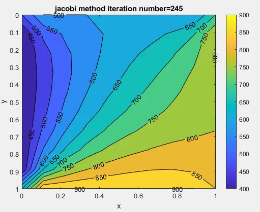
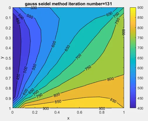
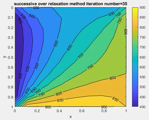
plots for temperature profiles of different itreative methods:

Although all the below plots look same but the number of iteration it took to reach the final state are different for every method

the least number of iterations were taken by sor method with relaxtion factor of 1.5.

sor method converges faster towards the solution because of using present time step value and relaxation factor .

number of nodes increases the number of iterations also increases.the below plots are generated for n=10;.

much smoother temperature profiles can be obtained by increasing the node points (n)

part 2

Theroy

if any property of sysytem varys with respect to time then it is defined as unsteady state of system

general 2-dimensional unsteady heat conduction equation

dT/dt=-b*(d^2T/dx^2 + d^2T/dy^2 );

b is thermal diffusivity m^2/sec if alpha is high then the medium quickly changes its temperature .hence less time is required to reach temperature

b = thermal condutivtiy/(density * specific heat);

applying central differencing scheme on right hand side the 2d heat conduction equation reduces to

t(i,j) =told(i,j)+k1*(told(i+1,j)-(2*told(i,j))+told(i-1,j))+k2*(told(i,j+1)-(2*told(i,j))+told(i,j-1));

k1=(b*dt)/(dx^2);
k2=(b*dt)/(dy^2);

b=thermal diffusivity

This code is for unsteady 2d heat conduction in explicit method

clear all
close all
clc
%inputs
l=1
nx=10;
ny=nx;
t=300*ones(nx,ny);
%assigning bc
t(:,nx)=800;
t(nx,:)=900;
t(1,:)=600;
t(:,1)=400;
t(1,nx)=(t(1,nx-1)+t(2,nx))/2;
t(nx,nx)=(t(nx,nx-1)+t(nx-1,nx))/2;
t(1,1)=(t(1,2)+t(2,1))/2;
t(nx,1)=(t(nx-1,1)+t(nx,2))/2;
%creating a copy of t
told=t;
x=linspace(0,1,nx);
y=linspace(0,1,ny);
dx=l/(nx-1);
dy=dx;
dt=1e-4;
b=1.4;%thermal diffusivity
k1=(b*dt)/(dx^2);
k2=(b*dt)/(dy^2);
cfl=k1+k2;
nt=1450;
for k=1:nt;
for i=2:nx-1;
for j=2:ny-1;
term1=k1*(told(i+1,j)-(2*told(i,j))+told(i-1,j));
term2=k2*(told(i,j+1)-(2*told(i,j))+told(i,j-1));
t(i,j)=told(i,j)+term1+term2;
end
end
told=t;
% plotting
figure(1)
contourf(x,y,t,'showtext','on');
set(gca,'yDIR','reverse')
colorbar
xlabel('x');
ylabel('y');
legend('2d unsteady explicit method');
pause(0.03)
end

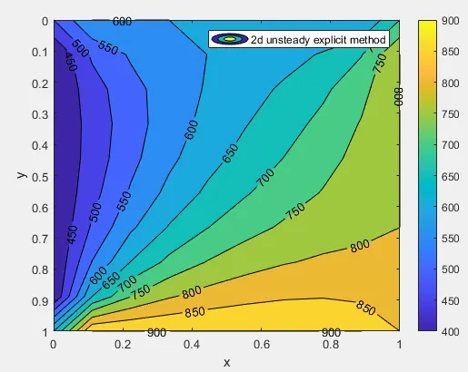
although the below plot is same as the steady state plot there is difference in solution .this plot is generated for 2d unsteady state heat conduction in explicit method .plot varys with respect to time (nt) value .if we set the nt value to 100 we can see the temperature profiles at 100th time step.initially the system will be under unsteady state so the temperature profiles varys rapidly with time after enoungh number of time steps the sytem reachs steady state there will not be any variation in temperature profiles

part 3

Theory

unsteady heat conduction equation can be solved in two ways explicit and implicit method . in implicit method we use different iterative method to calulate the temperture of all the nodes at newer time steps.

jacobi method

k1=(b*dt)/(dx^2);
k2=(b*dt)/(dy^2);

term1=1/(1+2*k1+2*k2);
term2=k1*term1;
term3=k2*term1

h=(told(i+1,j)+told(i-1,j));
v=(told(i,j+1)+told(i,j-1));
t(i,j)=tprev(i,j)*term1+term2*h+term3*v

gauss siedel method

h=(told(i+1,j)+t(i-1,j))
v=(told(i,j+1)+t(i,j-1))
t(i,j)=tprev(i,j)*term1+term2*h+term3*v

sor method

h=(told(i+1,j)+t(i-1,j))
v=(told(i,j+1)+t(i,j-1))
t(i,j)=(1-a)*tprev(i,j)+a*(tprev(i,j)*term1+term2*h+term3*v)

This code is for unsteady state 2d heat conduction in implicit method

clear all
close all
clc
%inputs
l=1
nx=10;
ny=nx;
t=300*ones(nx,ny);
%assigning bc
t(:,nx)=800;
t(nx,:)=900;
t(1,:)=600;
t(:,1)=400;
t(1,nx)=(t(1,nx-1)+t(2,nx))/2;
t(nx,nx)=(t(nx,nx-1)+t(nx-1,nx))/2;
t(1,1)=(t(1,2)+t(2,1))/2;
t(nx,1)=(t(nx-1,1)+t(nx,2))/2;
%creating a copy of t
told=t;
tprev=told;
x=linspace(0,1,nx);
y=linspace(0,1,ny);
dx=l/(nx-1);
dy=dx;
dt=1e-4;
b=1.4;%thermal diffusivity
a=1.2;%alpha
k1=(b*dt)/(dx^2);
k2=(b*dt)/(dy^2);
cfl=k1+k2;
term1=1/(1+2*k1+2*k2);
term2=k1*term1;
term3=k2*term1
nt=1450;
iterative_solver=3

%jacobi method
if iterative_solver==1

for k=1:nt;
error=6667;
tol=1e-5;
while(error>tol);

for i=2:nx-1;
for j=2:ny-1;
h=(told(i+1,j)+told(i-1,j));
v=(told(i,j+1)+told(i,j-1));
t(i,j)=tprev(i,j)*term1+term2*h+term3*v;
end
end
error=max(max(abs(told-t)));
told=t;

end
tprev=t;
contourf(x,y,t,'showtext','on');
set(gca,'yDIR','reverse')
colorbar
xlabel('x');
ylabel('y');
pause(0.03)

end

end

%gs method
if iterative_solver==2

for k=1:nt;
error=6667;
tol=1e-5;
while(error>tol);

for i=2:nx-1;
for j=2:ny-1;
h=(told(i+1,j)+t(i-1,j));
v=(told(i,j+1)+t(i,j-1));
t(i,j)=tprev(i,j)*term1+term2*h+term3*v;
end
end
error=max(max(abs(told-t)));
told=t;

end
tprev=t;
contourf(x,y,t,'showtext','on');
set(gca,'yDIR','reverse')
colorbar
xlabel('x');
ylabel('y');
pause(0.03)

end

end

%sor method
if iterative_solver==3

for k=1:nt;
error=6667;
tol=1e-5;
while(error>tol);

for i=2:nx-1;
for j=2:ny-1;
h=(told(i+1,j)+t(i-1,j));
v=(told(i,j+1)+t(i,j-1));
t(i,j)=(1-a)*tprev(i,j)+a*(tprev(i,j)*term1+term2*h+term3*v);
end
end
error=max(max(abs(told-t)));
told=t;

end
tprev=t;
contourf(x,y,t,'showtext','on');
set(gca,'yDIR','reverse')
colorbar
xlabel('x');
ylabel('y');
pause(0.03)

end

end

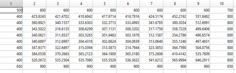
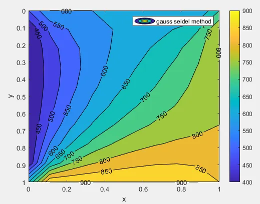
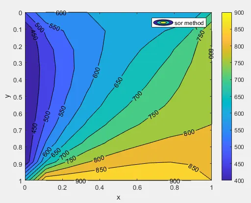
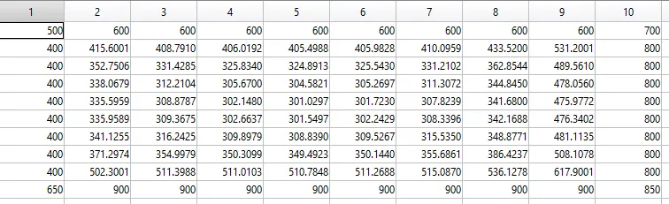
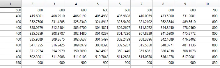
Although all the below plots look same but there is variation in them , to observ the variation calculate the temperature matrix after 50 time steps . if we observ the temperature matrix of jacobi and gauss siedel there is no variation but if we see the sor temperature matrix temperture at different nodes are different comparied to that of other method the temperture values are on higher side in sor method .it indicates that the in sor method the temperature of the nodes converge faster towards steady state

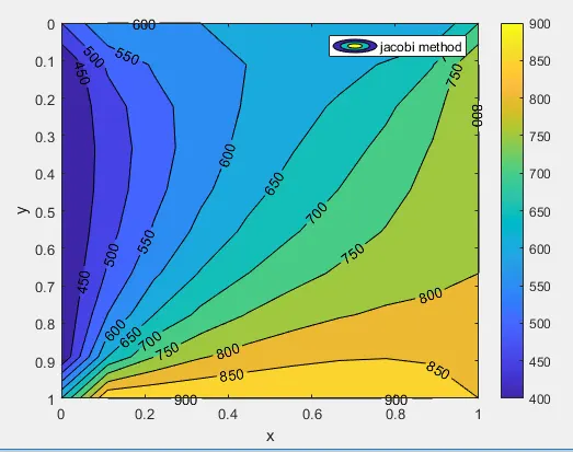
temperature (t) matrix of jacobi method after 50 time steps

temperature (t) matrix of gauss seidel method after 50 time steps

temperature(t) matrix of sor method after 50 time steps