Week 7 - Simulation of a 1D Super-sonic nozzle flow simulation using Macormack Method
OBJECTIVE:TO SIMULATE ISENTROPIC FLOW THROUGH A QUASI 1DIMENSIONAL SUBSONIC-SUPERSONIC NOZZLE.THIS SIMULATION IS USED TO OBSERVE THE VARATION OF PRIMITIVE VARIABLES IN NOZZLE AND COMPARE THE MASS FLOW RATE VARIATION WITH CONSERVATION AND NON-CONSERVATION FORM OF EQUATIONS.
THEORY
COMPRESSIBLE FLOWS
The flow is said to be compresssible when the density along the flow field is not constant (therefore the volume of the every portion of the fluid is constantly changing over the course of its motion) . compressiblity can be neglected when mach number less than 0.3.
Mach number =speed of flow/ speed of sound
speed of sound (C)=sqrt(gama*gas constant(R)*temperature(T)
if Mach number < 1 subsonic flow
mach number = 1 sonic flow
mach number > 1 supersonic flow
ISENTROPIC PROCESS
The entropy change in reversible process is defined as the ratio of change in heat energy to temperature .if the process is adibatic then the change in heat energy tends to zero and entropy is constant(S1=S2) in the process , such a process is called isentropic process .
if the process is reversible adibatic process then we can say that it is an isentropic process
MACORMACK METHOD FOR NON-CONSERVATION FORM
NON-CONSERVATION FORM OF EQUATIONS
Continutiy equation

Momentum equation

Energy equation

Predictor step
Continutiy equation

Momentum equation

Energy equation

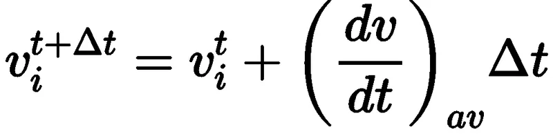
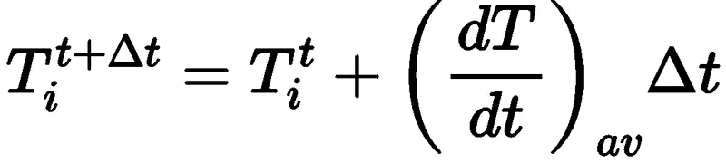
Intermediate solution update
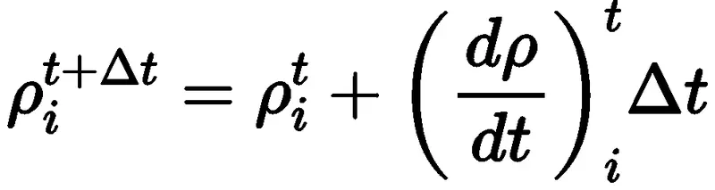
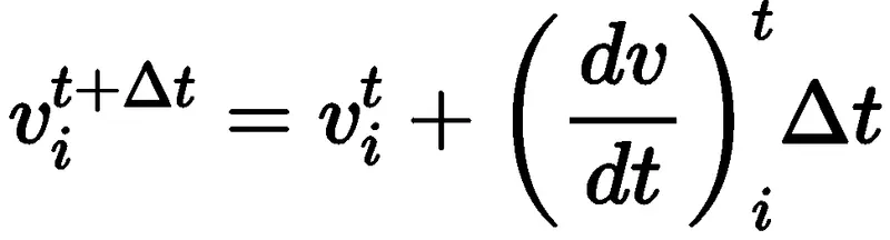
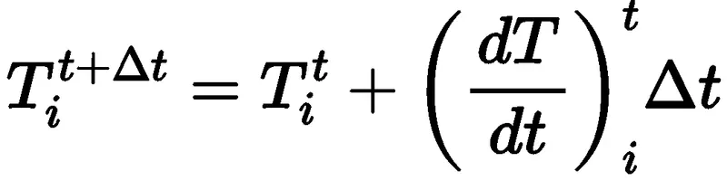
corrector step
Continutiy equation

Momentum equation

Energy equation

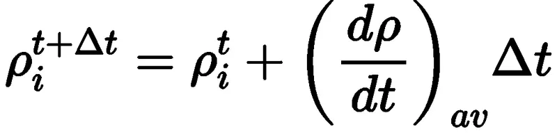
Average



Final solution update
MACORMACK METHOD FOR CONSERVATION FORM
CONSERVATION FORM OF EQUATIONS
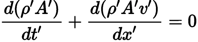
Continutiy equation
Momentum equation

Energy equation

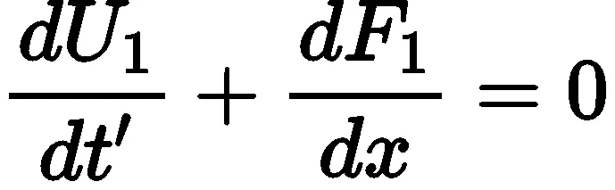
Continutiy equation interms of solution and flux vectors
Momentum equation interms of solution and flux vectors
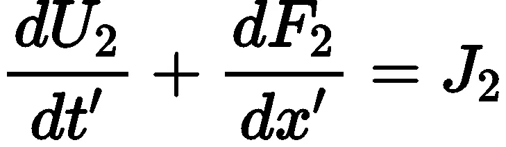
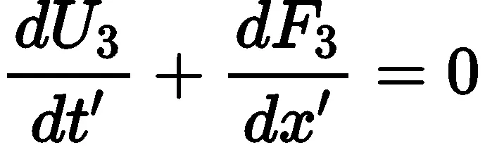
Energy equation interms of solution and flux vectors
INITIAL CONDITIONS

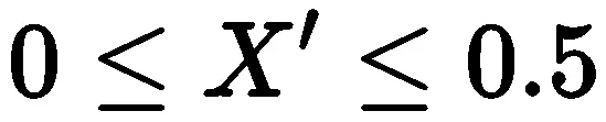
ρ'=1
T'=1






Primitive variables interms of solution vector terms
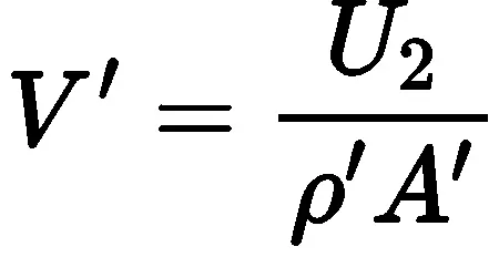

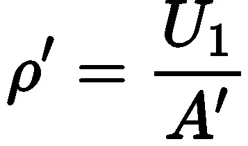
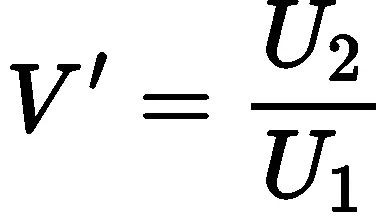
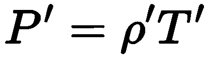
Relation between solution vector and primitive variables
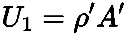
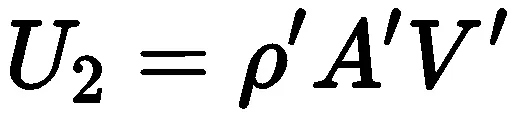
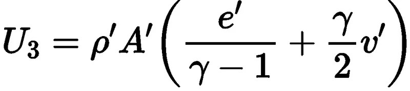
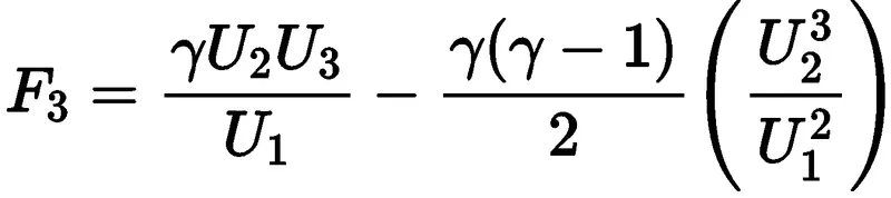
Relation between solution vectors terms and flux vecctor terms
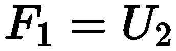

Source term

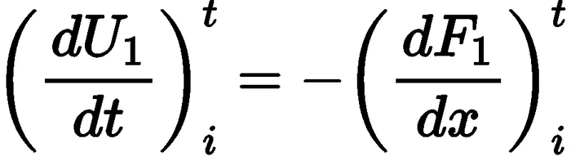
Continutiy equation interms of solution and flux vectors
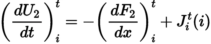
Momentum equation interms of solution and flux vectors
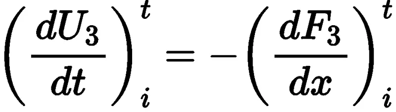
Energy equation interms of solution and flux vectors
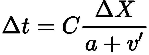
predictor step
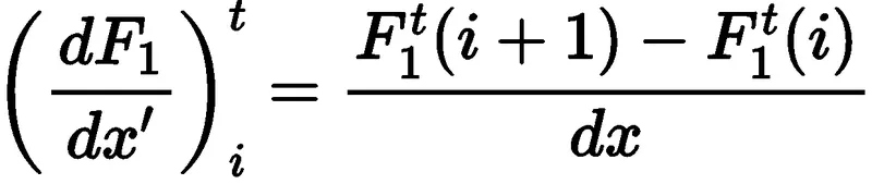
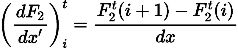
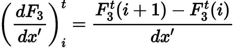
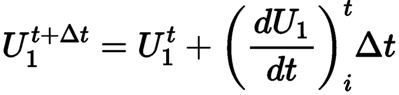
Intermediate Solution vector Update
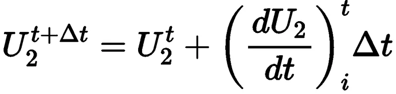
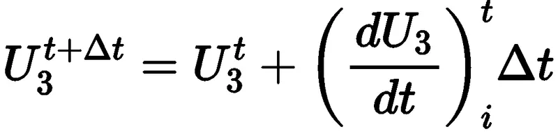
Corrector step




Average of time derivative of solution vector



Final update of solution vector
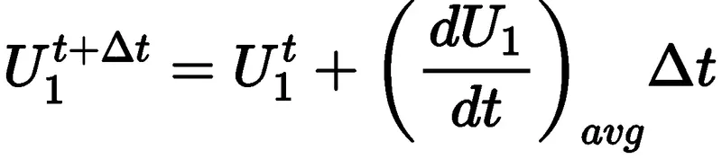
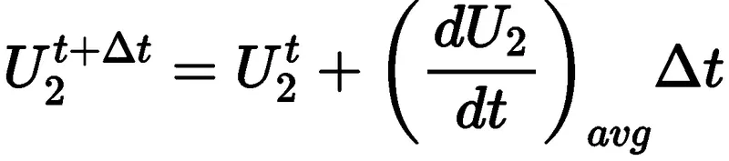
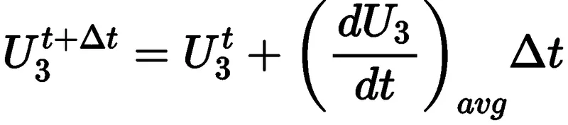
Final update of primitive variables
CODE FOR NON CONSERVATIVE FORM
close all
clear all
clc
%inputs
n=31; %number of grid points
x=linspace(0,3,n);
dx=x(2)-x(1);
%initial primitive variables
rho_nc=1-0.3146*x; %density
t_nc=1-0.2314*x; %temperature
v_nc=(0.1+1.09*x).*(t_nc.^0.5); %velocity
a=1+(2.2*((x-1.5).^2)); % area profile of the nozzle
gamma=1.4; %ratio of specific heats
throat=(n+1)/2; %throat location
%macormack method for non-conservation form
%time steps
nt=1400;
dt=min((0.5*dx)./(t_nc.^(1/2)+v_nc));
tic
%outer time loop
for k=1:nt
rho_old=rho_nc;
v_old=v_nc;
t_old=t_nc;
%predictor step
for j=2:n-1
drhodx=(rho_nc(j+1)-rho_nc(j))/dx;
dvdx=(v_nc(j+1)-v_nc(j))/dx;
dtdx=(t_nc(j+1)-t_nc(j))/dx;
dlogadx=(log(a(j+1))-log(a(j)))/dx;
%continuty equation
drhodt_p(j)=-(rho_nc(j)*dvdx)-(rho_nc(j)*v_nc(j)*dlogadx)-(v_nc(j)*drhodx);
%momentum equation
dvdt_p(j)=-(v_nc(j)*dvdx)-((1/gamma)*(dtdx+(t_nc(j)/rho_nc(j))*drhodx));
%energy equation
dtdt_p(j)=-(v_nc(j)*dtdx)-((gamma-1)*t_nc(j)*(dvdx+v_nc(j)*dlogadx));
%updating the primitive variables after predictor step
rho_nc(j)=rho_nc(j)+drhodt_p(j)*dt;
v_nc(j)=v_nc(j)+dvdt_p(j)*dt;
t_nc(j)=t_nc(j)+dtdt_p(j)*dt;
end
%corrector step
for j=2:n-1
drhodx=(rho_nc(j)-rho_nc(j-1))/dx;
dvdx=(v_nc(j)-v_nc(j-1))/dx;
dtdx=(t_nc(j)-t_nc(j-1))/dx;
dlogadx=(log(a(j))-log(a(j-1)))/dx;
%continuty equation
drhodt_c(j)=-(rho_nc(j)*dvdx)-(rho_nc(j)*v_nc(j)*dlogadx)-(v_nc(j)*drhodx);
%momentum equation
dvdt_c(j)=-(v_nc(j)*dvdx)-((1/gamma)*(dtdx+(t_nc(j)/rho_nc(j))*drhodx));
%energy equation
dtdt_c(j)=-(v_nc(j)*dtdx)-((gamma-1)*t_nc(j)*(dvdx+v_nc(j)*dlogadx));
end
%calculating average time derivatives of primitive variables
drhodt=0.5*(drhodt_p+drhodt_c);
dvdt=0.5*(dvdt_p+dvdt_c);
dtdt=0.5*(dtdt_p+dtdt_c);
%final update of primitive variables
for i=2:n-1
rho_nc(i)=rho_old(i)+drhodt(i)*dt;
v_nc(i)=v_old(i)+dvdt(i)*dt;
t_nc(i)=t_old(i)+dtdt(i)*dt;
end
%boundary conditions for inlet & outlet
%inlet
v_nc(1)=2*v_nc(2)-v_nc(3);
rho_nc(1)=1;
t_nc(1)=1;
%outlet
v_nc(n)=2*v_nc(n-1)-v_nc(n-2);
rho_nc(n)=2*rho_nc(n-1)-rho_nc(n-2);
t_nc(n)=2*t_nc(n-1)-t_nc(n-2);
mf_nc=rho_nc.*a.*v_nc;
p_nc=rho_nc.*t_nc;
mac_nc=v_nc./(t_nc).^1/2;
counter=toc;
%claculation of primitive variables at throat of the nozzle
p_t_nc(k)=p_nc(throat);
t_t_nc(k)=t_nc(throat);
rho_t_nc(k)=rho_nc(throat);
mac_t_nc(k)=mac_nc(throat);
mf_t_nc(k)=mf_nc(throat);
% ploting massflow rate vs length of the nozzle
figure(1)
hold on
if k==50
plot(x,mf_nc,'b','linewidth',2)
xlabel ('length of nozzle')
ylabel('massflow rate')
elseif k==100
plot(x,mf_nc,'r','linewidth',2)
elseif k==150
plot(x,mf_nc,'m','linewidth',2)
elseif k==200
plot(x,mf_nc,'k','linewidth',2)
elseif k==700
plot(x,mf_nc,'y','linewidth',2)
elseif k==1000
plot(x,mf_nc,'g','linewidth',2)
legend('k=50','k=100','k=150','k=200','k=700','k=1000')
title(sprintf('NON CONSERVATION FORM TIME=%f s',counter))
end
%plots for the variation of the primitive variables
figure(2)
subplot(4,1,1)
plot(p_t_nc,'r','linewidth',2)
ylabel('p/po')
title(sprintf('NON CONSERVATION FORM TIME=%f s',counter))
subplot(4,1,2)
plot(t_t_nc,'b','linewidth',2)
ylabel('t/to')
subplot(4,1,3)
plot(rho_t_nc,'y','linewidth',2)
ylabel('rho/rho0')
subplot(4,1,4)
plot(mac_t_nc,'k','linewidth',2)
ylabel('mach no')
xlabel('no of iterations')
%ploting primitive varibales vs length of the nozzle
figure(3)
subplot(4,1,1)
plot(x,mac_nc,'r','linewidth',2)
ylabel('M')
title(sprintf('NON CONSERVATION FORM TIME=%f s',counter))
subplot(4,1,2)
plot(x,p_nc,'b','linewidth',2)
ylabel('p/po')
subplot(4,1,3)
plot(x,t_nc,'g','linewidth',2)
ylabel('t/to')
subplot(4,1,4)
plot(x,rho_nc,'m','linewidth',2)
xlabel('x/l')
ylabel('rho/rho0')
%ploting massflow rate vs length of the nozzle
figure(4)
plot(x,mf_nc,'b','linewidth',2)
xlabel('length of nozzle')
ylabel('massflow rate')
legend('non-conservative form')
title(sprintf('NON CONSERVATION FORM TIME=%f s',counter))
figure(5)
plot(mf_t_nc,'r','linewidth',2)
xlabel('no of iteratons')
ylabel('massflow rate')
legend('non-conservative form')
title(sprintf('NON CONSERVATION FORM TIME=%f s',counter))
end
RESULTS OF NON-CONSERVATION FORM AT 31 GRID POINTS
Figure 1
The below plot represents massflow rate verus length of the nozzle at different time steps as we colud see that initally the massflow rate varies upto 700 time step and after 1000th timpe step massflow rate reachs steady state and there no varition in mass floe rate after 1000 timesteps(generally the massflow rate controlled by back pressure at the exit of the nozzle by decreasing the back pressure massflow rate can be increased but at some point futher reduction in back pressure will not increase the massflow rate it remains constant this flow is called choked flow)
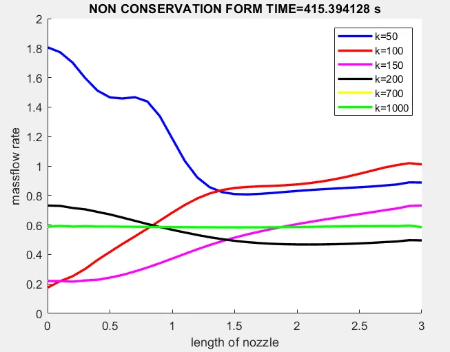
Figure 2
The below plot represents variation of primitive variables(density,pressure,temperature and mach number) withrespect no of iterations, after 600 time steps the primitive variables slope is zero and its values are constant
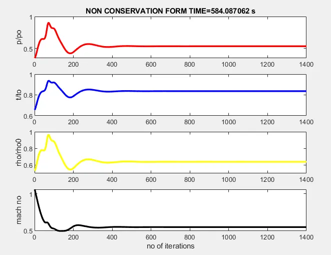
Figure 3
The below plot represents variation of primitive variables(density,pressure,temperature and mach number) withrespect length of the nozzle, (0-1.5) is the convergent section,(1.5-3) is the divergent section and (1.5) the throat section . in any covergent section we cannot accelerate the flow above sonic speed ,to accelerate the flow above sonic speed (mac>1) we sholud use both convergent and divergent section .at the end of convergent section flow can be accelerated to sonic speed(mac=1) after that in the divergent section the flow is futher more accelerated to supersonic flow(mac>1).because of that mac no increases along the length of the nozzzle
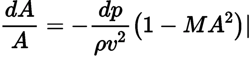
The above relation is for isentropic flow in ducts since it describes the the variation of pressure with flow area .
for subsonic flow (ma<1) the term (1-Ma^2) is positive and thus dA and dP must have same signs .that is pressure of the fluid must increase as the flow area of the duct increses and must decrease as the flow area decreases thus at subsonic velocities the pressure decreases in converging ducts and increases in diverging ducts
for supersonic flow (ma>1) the term (1-Ma^2) is negtive and thus dA and dP must have opposite signs that is the pressure of the fluid must increase as the flow area of the duct decreasses aand must decrease as the flow area of the duct increases .thus at supersonic velocities the pressure decreases in diverging ducts and increases in converging ducts
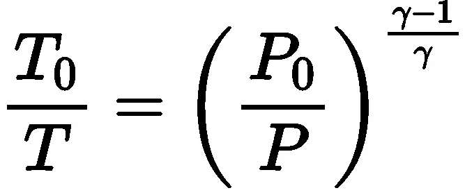
The above relation is for isentropic flow in ducts since it describes the the variation of temperature ratio with pressure ratio .based on the increase or decrease in pressure ratio the the temperature ratio increase or decrease respectively
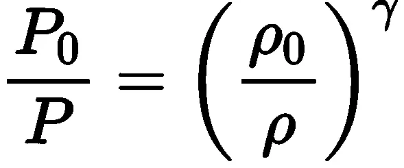
The above relation is for isentropic flow in ducts since it describes the the variation of density ratio with presssure .based on the increase or decrease in pressure ratio the the density ratio increase or decrease respectively
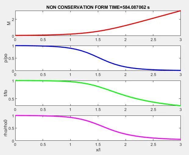
Figure 4
The below plot represents variation of massflow rate verus length of the nozzle
Generally the massflow rate controlled by back pressure at the exit of the nozzle by decreasing the back pressure massflow rate can be increased but at some point futher reduction in back pressure will not increase the massflow rate it remains constant this flow is called choked flow. in this case the back pressure is constant so the slope massflow rate variation with respect to length of the nozzle sholud be zero (means a straight line parallel to x axis) because of the numerical computation of massflow rate there is a deviation form actual plot in non conservation form
the mass flow rate value fluctuates between minimum of 0.584 to maximumu of 0.594
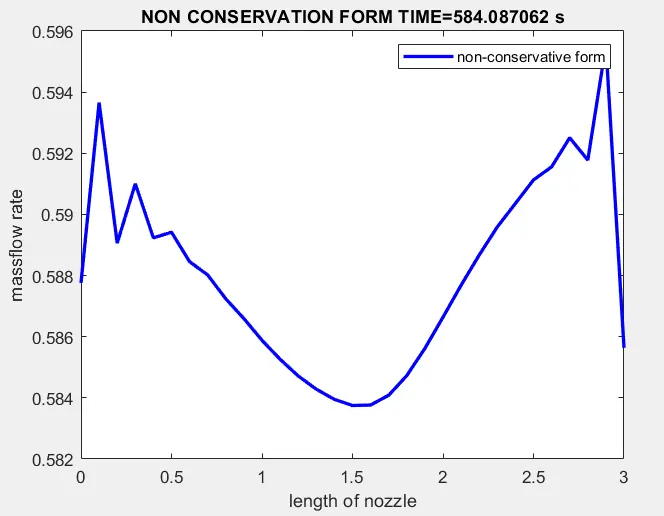
Figure 5
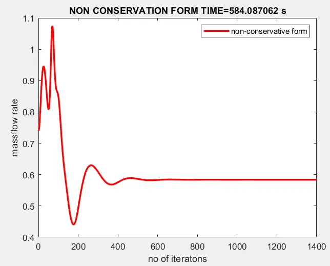
The below plot represents variation of massflow rate verus no of iterations
the below plot clearly indicates after 600 time steps the mass flow rate variation reachs steady state futher there is no variation in massflow rate
CODE FOR CONSERVATION FORM
close all
clear all
clc
%generating grid points
n=31; % number of grid points
x=linspace(0,3,n);
dx=x(2)-x(1);
%initializing the primitive variables
a=1+2.2.*(x-1.5).^2; %area profile of nozzle
g=1.4; %ratio of specific heats gamma
throat=(n+1)/2; %location of throat
%intinal conditions for primitive variables
for i=1:n
if (x(i)>=0 && x(i)<=0.5)
rho(i)=1; %density
t(i)=1; %temperature
elseif(x(i)>0.5 && x(i)<=1.5)
rho(i)=1-0.366*(x(i)-0.5);
t(i)=1-0.167*(x(i)-0.5);
elseif (x(i)>1.5 && x(i)<=3.5)
rho(i)=0.634-0.3879*(x(i)-1.5);
t(i)=0.833-0.3507*(x(i)-1.5);
end
end
%calculating initial solution vector
v=0.59./(rho.*a); % velocity
u1=rho.*a;
u2= rho.*a.*v;
u3=rho.*a.*((t./(g-1))+(g*v*0.5));
%macormack method for conservation form
nt=1400;
tic
%time loop
for k=1:nt;
u1_old=u1;
u2_old=u2;
u3_old=u3;
dt=min((0.5*dx)./(sqrt(t)+v));
%calculating flux vector
f1=u2;
f2=(u2.^2./u1)+( (g-1)/g)*(u3-(g*0.5)*(u2.^2./u1));
f3=((g*u2.*u3)./u1)-(g*(g-1)*0.5*(u2.^3/u1.^2));
%predictor step
for j=2:n-1;
%source trem
dadx=(a(j+1)-a(j))/dx;
j2=(1/g)*rho(j)*t(j)*dadx; %soure term
%continuty equation
du1dt_p(j)=-(f1(j+1)-f1(j))/dx;
%momentum equation
du2dt_p(j)=-((f2(j+1)-f2(j))/dx)+j2;
%energy equation
du3dt_p(j)=-(f3(j+1)-f3(j))/dx;
%updating solution vector
u1(j)=u1_old(j)+du1dt_p(j)*dt;
u2(j)=u2_old(j)+du2dt_p(j)*dt;
u3(j)=u3_old(j)+du3dt_p(j)*dt;
end
%updating the primitive varaibles after predictor step
rho=u1./a;
v=u2./u1;
t=(g-1)*((u3./u1)-g*0.5.*v);
%updating flux terms after predictor step
f1=u2;
f2=(u2.^2./u1)+( (g-1)/g)*(u3-(g*0.5)*(u2.^2./u1));
f3=((g*u2.*u3)./u1)-(g*(g-1)*0.5*((u2.^3)./(u1.^2)));
% corrector step
for j=2:n-1;
dadx=(a(j)-a(j-1))/dx;
j2=(1/g)*rho(j)*t(j)*dadx;
%continuty equation
du1dt_c(j)=-(f1(j)-f1(j-1))/dx;
%momentum equation
du2dt_c(j)=-((f2(j)-f2(j-1))/dx)+j2;
%energy equation
du3dt_c(j)=-(f3(j)-f3(j-1))/dx;
end
%calculating average time derivatives of solution vectors
du1dt=0.5*(du1dt_c+du1dt_p);
du2dt=0.5*(du2dt_c+du2dt_p);
du3dt=0.5*(du3dt_c+du3dt_p);
%final update of solution vectors
for i=1:n-1;
u1(i)=u1_old(i)+du1dt(i)*dt;
u2(i)=u2_old(i)+du2dt(i)*dt;
u3(i)=u3_old(i)+du3dt(i)*dt;
end
%boundary conditions for inlet & outlet
%inlet condition
u1(1)=rho(1)*a(1);
u2(1)=2*u2(2)-u2(3);
u3(1)=u1(1)*((t(1)/(g-1))+g*0.5*v(1));
%outlet conditions
u1(n)=2*u1(n-1)-u1(n-2);
u2(n)=2*u2(n-1)-u2(n-2);
u3(n)=2*u3(n-1)-u3(n-2);
%calculating final values of primitive variables
rho=u1./a;
v=u2./u1;
t=(g-1)*((u3./u1)-g*0.5.*v);
mf=u2;
p=rho.*t;
mac=v./((t).^1/2);
counter=toc;
%claculation of primitive variables at throat of the nozzle
p_t(k)=p(throat);
t_t(k)=t(throat);
rho_t(k)=rho(throat);
mac_t(k)=mac(throat);
mf_t(k)=mf(throat);
% ploting massflow rate vs length of the nozzle
figure(1)
hold on
if k==50
plot(x,mf,'b','linewidth',2)
xlabel ('length of nozzle')
ylabel('massflow rate')
elseif k==100
plot(x,mf,'r','linewidth',2)
elseif k==150
plot(x,mf,'m','linewidth',2)
elseif k==200
plot(x,mf,'k','linewidth',2)
elseif k==700
plot(x,mf,'y','linewidth',2)
elseif k==1000
plot(x,mf,'g','linewidth',2)
legend('k=50','k=100','k=150','k=200','k=700','k=1000')
title(sprintf('CONSERVATION FORM TIME=%f s',counter))
end
%plots for the variation of the primitive variables
figure(2)
subplot(4,1,1)
plot(p_t,'r','linewidth',2)
ylabel('p/po')
title(sprintf('CONSERVATION FORM TIME=%f s',counter))
subplot(4,1,2)
plot(t_t,'b','linewidth',2)
ylabel('t/to')
subplot(4,1,3)
plot(rho_t,'y','linewidth',2)
ylabel('rho/rho0')
subplot(4,1,4)
plot(mac_t,'k','linewidth',2)
ylabel('mach no')
xlabel('no of iterations')
%ploting primitive varibales vs length of the nozzle
figure(3)
subplot(4,1,1)
plot(x,mac,'r','linewidth',2)
ylabel('M')
title(sprintf('CONSERVATION FORM TIME=%f s',counter))
subplot(4,1,2)
plot(x,p,'b','linewidth',2)
ylabel('p/po')
subplot(4,1,3)
plot(x,t,'g','linewidth',2)
ylabel('t/to')
subplot(4,1,4)
plot(x,rho,'m','linewidth',2)
xlabel('x/l')
ylabel('rho/rho0')
%ploting massflow rate vs length of the nozzle
figure(4)
plot(x,mf,'b','linewidth',2)
xlabel('length of nozzle')
ylabel('massflow rate')
legend('CONSERVATION FORM')
title(sprintf('CONSERVATION FORM TIME=%f s',counter))
figure(5)
plot(mf_t,'r','linewidth',2)
xlabel('no of iteratons')
ylabel('massflow rate')
legend('conservative form')
title(sprintf('CONSERVATION FORM TIME=%f s',counter))
end
RESULTS FOR CONSERVATION FORM WITH 31 GRID POINTS
Figure 6
The below plot represents massflow rate verus length of the nozzle at different time steps as we colud see that initally the massflow rate varies upto 700 time step and after 1000th timpe step massflow rate reachs steady state and there no varition in mass floe rate after 1000 timesteps
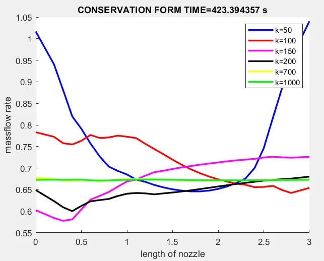
Figure 7
The below plot represents variation of primitive variables(density,pressure,temperature and mach number) withrespect no of iterations, after 1000 time steps the primitive variables fluctuation are considerably reduced reachs a constant value.
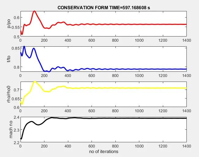
Figure 8
The below plot represents variation of primitive variables(density,pressure,temperature and mach number) withrespect length of the nozzle, (0-1.5) is the convergent section,(1.5-3) is the divergent section and (1.5) the throat section . in any covergent section we cannot accelerate the flow above sonic speed ,to accelerate the flow above sonic speed (mac>1) we sholud use both convergent and divergent section .at the end of convergent section flow can be accelerated to sonic speed(mac=1) after that in the divergent section the flow is futher more accelerated to supersonic flow(mac>1).because of that mac no increases along the length of the nozzzle
The above relation is for isentropic flow in ducts since it describes the the variation of pressure with flow area .
for subsonic flow (ma<1) the term (1-Ma^2) is positive and thus dA and dP must have same signs .that is pressure of the fluid must increase as the flow area of the duct increses and must decrease as the flow area decreases thus at subsonic velocities the pressure decreases in converging ducts and increases in diverging ducts
for supersonic flow (ma>1) the term (1-Ma^2) is negtive and thus dA and dP must have opposite signs that is the pressure of the fluid must increase as the flow area of the duct decreasses aand must decrease as the flow area of the duct increases .thus at supersonic velocities the pressure decreases in diverging ducts and increases in converging ducts
The above relation is for isentropic flow in ducts since it describes the the variation of temperature ratio with pressure ratio .based on the increase or decrease in pressure ratio the the temperature ratio increase or decrease respectively
The above relation is for isentropic flow in ducts since it describes the the variation of density ratio with presssure .based on the increase or decrease in pressure ratio the the density ratio increase or decrease respectively
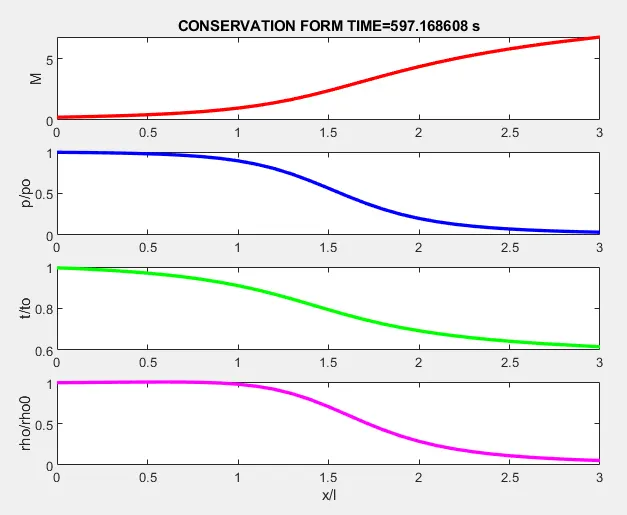
Figure 9
The below plot represents variation of massflow rate verus length of the nozzle
Generally the massflow rate controlled by back pressure at the exit of the nozzle by decreasing the back pressure massflow rate can be increased but at some point futher reduction in back pressure will not increase the massflow rate it remains constant this flow is called choked flow. in this case the back pressure is constant so the slope massflow rate variation with respect to length of the nozzle sholud be zero (means a straight line parallel to x axis) because of the numerical computation of massflow rate there is a deviation form actual plot in conservation form
the mass flow rate value fluctuates between minimum of 0.6717 to maximumu of 0.6733
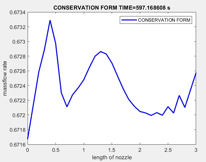
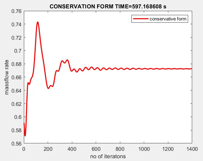
Figure 10
The below plot represents variation of massflow rate verus no of iterations
the below plot clearly indicates after 600 time steps the mass flow rate fluctuates betwween 0.67 t0 0.68
MAIN PROGRAM FOR BOTH CONSERVATION AND NON CONSERVATION
close all
clear all
clc
%generating grid points
n=31; % number of grid points
x=linspace(0,3,n);
dx=x(2)-x(1);
%initializing the primitive variables
a=1+2.2.*(x-1.5).^2; %area profile of nozzle
g=1.4; %ratio of specific heats gamma
throat=(n+1)/2; %location of throat
nt=1400; %no of time steps
%conservation form
[rho,v,t,mac,mf,rho_t,t_t,mac_t,mf_t,p,p_t]=conservation_fun(x,a,n,nt,dx,g,throat);
%non conservation form
[rho_nc,t_nc,v_nc,mac_nc,mf_nc,p_nc,rho_t_nc,p_t_nc,t_t_nc,mac_t_nc,mf_t_nc]=non_conservation_fun(x,a,n,nt,dx,g,throat);
figure(11)
plot(x,mf,'r',x,mf_nc,'b','linewidth',2)
xlabel('length of nozzle')
ylabel('massflow rate')
legend('conseravtion_form','non_conseravtion_form')
FUNCTION FOR CONSERVATION FORM
function [rho,v,t,mac,mf,rho_t,t_t,mac_t,mf_t,p,p_t]=conservation_fun(x,a,n,nt,dx,g,throat)
%intinal conditions for primitive variablest
for i=1:n
if (x(i)>=0 && x(i)<=0.5)
rho(i)=1; %density
t(i)=1; %temperature
elseif(x(i)>0.5 && x(i)<=1.5)
rho(i)=1-0.366*(x(i)-0.5);
t(i)=1-0.167*(x(i)-0.5);
elseif (x(i)>1.5 && x(i)<=3.5)
rho(i)=0.634-0.3879*(x(i)-1.5);
t(i)=0.833-0.3507*(x(i)-1.5);
end
end
%calculating initial solution vector
v=0.59./(rho.*a); % velocity
u1=rho.*a;
u2= rho.*a.*v;
u3=rho.*a.*((t./(g-1))+(g*v*0.5));
%macormack method for conservation form
nt=1400;
tic
%time loop
for k=1:nt;
u1_old=u1;
u2_old=u2;
u3_old=u3;
dt=min((0.5*dx)./(sqrt(t)+v));
%calculating flux vector
f1=u2;
f2=(u2.^2./u1)+( (g-1)/g)*(u3-(g*0.5)*(u2.^2./u1));
f3=((g*u2.*u3)./u1)-(g*(g-1)*0.5*(u2.^3/u1.^2));
%predictor step
for j=2:n-1;
%source trem
dadx=(a(j+1)-a(j))/dx;
j2=(1/g)*rho(j)*t(j)*dadx; %soure term
%continuty equation
du1dt_p(j)=-(f1(j+1)-f1(j))/dx;
%momentum equation
du2dt_p(j)=-((f2(j+1)-f2(j))/dx)+j2;
%energy equation
du3dt_p(j)=-(f3(j+1)-f3(j))/dx;
%updating solution vector
u1(j)=u1_old(j)+du1dt_p(j)*dt;
u2(j)=u2_old(j)+du2dt_p(j)*dt;
u3(j)=u3_old(j)+du3dt_p(j)*dt;
end
%updating the primitive varaibles after predictor step
rho=u1./a;
v=u2./u1;
t=(g-1)*((u3./u1)-g*0.5.*v);
%updating flux terms after predictor step
f1=u2;
f2=(u2.^2./u1)+( (g-1)/g)*(u3-(g*0.5)*(u2.^2./u1));
f3=((g*u2.*u3)./u1)-(g*(g-1)*0.5*((u2.^3)./(u1.^2)));
% corrector step
for j=2:n-1;
dadx=(a(j)-a(j-1))/dx;
j2=(1/g)*rho(j)*t(j)*dadx;
%continuty equation
du1dt_c(j)=-(f1(j)-f1(j-1))/dx;
%momentum equation
du2dt_c(j)=-((f2(j)-f2(j-1))/dx)+j2;
%energy equation
du3dt_c(j)=-(f3(j)-f3(j-1))/dx;
end
%calculating average time derivatives of solution vectors
du1dt=0.5*(du1dt_c+du1dt_p);
du2dt=0.5*(du2dt_c+du2dt_p);
du3dt=0.5*(du3dt_c+du3dt_p);
%final update of solution vectors
for i=1:n-1;
u1(i)=u1_old(i)+du1dt(i)*dt;
u2(i)=u2_old(i)+du2dt(i)*dt;
u3(i)=u3_old(i)+du3dt(i)*dt;
end
%boundary conditions for inlet & outlet
%inlet condition
u1(1)=rho(1)*a(1);
u2(1)=2*u2(2)-u2(3);
u3(1)=u1(1)*((t(1)/(g-1))+g*0.5*v(1));
%outlet conditions
u1(n)=2*u1(n-1)-u1(n-2);
u2(n)=2*u2(n-1)-u2(n-2);
u3(n)=2*u3(n-1)-u3(n-2);
%calculating final values of primitive variables
rho=u1./a;
v=u2./u1;
t=(g-1)*((u3./u1)-g*0.5.*v);
mf=u2;
p=rho.*t;
mac=v./((t).^1/2);
counter=toc;
%claculation of primitive variables at throat of the nozzle
p_t(k)=p(throat);
t_t(k)=t(throat);
rho_t(k)=rho(throat);
mac_t(k)=mac(throat);
mf_t(k)=mf(throat);
% ploting massflow rate vs length of the nozzle
figure(1)
hold on
if k==50
plot(x,mf,'b','linewidth',2)
xlabel ('length of nozzle')
ylabel('massflow rate')
elseif k==100
plot(x,mf,'r','linewidth',2)
elseif k==150
plot(x,mf,'m','linewidth',2)
elseif k==200
plot(x,mf,'k','linewidth',2)
elseif k==700
plot(x,mf,'y','linewidth',2)
elseif k==1000
plot(x,mf,'g','linewidth',2)
legend('k=50','k=100','k=150','k=200','k=700','k=1000')
title(sprintf('CONSERVATION FORM TIME=%f s',counter))
end
%plots for the variation of the primitive variables
figure(2)
subplot(4,1,1)
plot(p_t,'r','linewidth',2)
ylabel('p/po')
title(sprintf('CONSERVATION FORM TIME=%f s',counter))
subplot(4,1,2)
plot(t_t,'b','linewidth',2)
ylabel('t/to')
subplot(4,1,3)
plot(rho_t,'y','linewidth',2)
ylabel('rho/rho0')
subplot(4,1,4)
plot(mac_t,'k','linewidth',2)
ylabel('mach no')
xlabel('no of iterations')
%ploting primitive varibales vs length of the nozzle
figure(3)
subplot(4,1,1)
plot(x,mac,'r','linewidth',2)
ylabel('M')
title(sprintf('CONSERVATION FORM TIME=%f s',counter))
subplot(4,1,2)
plot(x,p,'b','linewidth',2)
ylabel('p/po')
subplot(4,1,3)
plot(x,t,'g','linewidth',2)
ylabel('t/to')
subplot(4,1,4)
plot(x,rho,'m','linewidth',2)
xlabel('x/l')
ylabel('rho/rho0')
%ploting massflow rate vs length of the nozzle
figure(4)
plot(x,mf,'b','linewidth',2)
xlabel('length of nozzle')
ylabel('massflow rate')
legend('CONSERVATION FORM')
title(sprintf('CONSERVATION FORM TIME=%f s',counter))
figure(5)
plot(mf_t,'r','linewidth',2)
xlabel('no of iteratons')
ylabel('massflow rate')
legend('conservative form')
title(sprintf('CONSERVATION FORM TIME=%f s',counter))
end
end
FUNCTION FOR NON-CONSERVATION FORM
function [rho_nc,t_nc,v_nc,mac_nc,mf_nc,p_nc,rho_t_nc,p_t_nc,t_t_nc,mac_t_nc,mf_t_nc]=non_conservation_fun(x,a,n,nt,dx,g,throat)
rho_nc=1-0.3146*x; %density
t_nc=1-0.2314*x; %temperature
v_nc=(0.1+1.09*x).*(t_nc.^0.5); %velocity
dt=min((0.5*dx)./(t_nc.^(1/2)+v_nc));
tic
%outer time loop
for k=1:nt
rho_old=rho_nc;
v_old=v_nc;
t_old=t_nc;
%predictor step
for j=2:n-1
drhodx=(rho_nc(j+1)-rho_nc(j))/dx;
dvdx=(v_nc(j+1)-v_nc(j))/dx;
dtdx=(t_nc(j+1)-t_nc(j))/dx;
dlogadx=(log(a(j+1))-log(a(j)))/dx;
%continuty equation
drhodt_p(j)=-(rho_nc(j)*dvdx)-(rho_nc(j)*v_nc(j)*dlogadx)-(v_nc(j)*drhodx);
%momentum equation
dvdt_p(j)=-(v_nc(j)*dvdx)-((1/g)*(dtdx+(t_nc(j)/rho_nc(j))*drhodx));
%energy equation
dtdt_p(j)=-(v_nc(j)*dtdx)-((g-1)*t_nc(j)*(dvdx+v_nc(j)*dlogadx));
%updating the primitive variables after predictor step
rho_nc(j)=rho_nc(j)+drhodt_p(j)*dt;
v_nc(j)=v_nc(j)+dvdt_p(j)*dt;
t_nc(j)=t_nc(j)+dtdt_p(j)*dt;
end
%corrector step
for j=2:n-1
drhodx=(rho_nc(j)-rho_nc(j-1))/dx;
dvdx=(v_nc(j)-v_nc(j-1))/dx;
dtdx=(t_nc(j)-t_nc(j-1))/dx;
dlogadx=(log(a(j))-log(a(j-1)))/dx;
%continuty equation
drhodt_c(j)=-(rho_nc(j)*dvdx)-(rho_nc(j)*v_nc(j)*dlogadx)-(v_nc(j)*drhodx);
%momentum equation
dvdt_c(j)=-(v_nc(j)*dvdx)-((1/g)*(dtdx+(t_nc(j)/rho_nc(j))*drhodx));
%energy equation
dtdt_c(j)=-(v_nc(j)*dtdx)-((g-1)*t_nc(j)*(dvdx+v_nc(j)*dlogadx));
end
%calculating average time derivatives of primitive variables
drhodt=0.5*(drhodt_p+drhodt_c);
dvdt=0.5*(dvdt_p+dvdt_c);
dtdt=0.5*(dtdt_p+dtdt_c);
%final update of primitive variables
for i=2:n-1
rho_nc(i)=rho_old(i)+drhodt(i)*dt;
v_nc(i)=v_old(i)+dvdt(i)*dt;
t_nc(i)=t_old(i)+dtdt(i)*dt;
end
%boundary conditions for inlet & outlet
%inlet
v_nc(1)=2*v_nc(2)-v_nc(3);
rho_nc(1)=1;
t_nc(1)=1;
%outlet
v_nc(n)=2*v_nc(n-1)-v_nc(n-2);
rho_nc(n)=2*rho_nc(n-1)-rho_nc(n-2);
t_nc(n)=2*t_nc(n-1)-t_nc(n-2);
mf_nc=rho_nc.*a.*v_nc;
p_nc=rho_nc.*t_nc;
mac_nc=v_nc./(t_nc).^1/2;
counter=toc;
%claculation of primitive variables at throat of the nozzle
p_t_nc(k)=p_nc(throat);
t_t_nc(k)=t_nc(throat);
rho_t_nc(k)=rho_nc(throat);
mac_t_nc(k)=mac_nc(throat);
mf_t_nc(k)=mf_nc(throat);
% ploting massflow rate vs length of the nozzle
figure(6)
hold on
if k==50
plot(x,mf_nc,'b','linewidth',2)
xlabel ('length of nozzle')
ylabel('massflow rate')
elseif k==100
plot(x,mf_nc,'r','linewidth',2)
elseif k==150
plot(x,mf_nc,'m','linewidth',2)
elseif k==200
plot(x,mf_nc,'k','linewidth',2)
elseif k==700
plot(x,mf_nc,'y','linewidth',2)
elseif k==1000
plot(x,mf_nc,'g','linewidth',2)
legend('k=50','k=100','k=150','k=200','k=700','k=1000')
title(sprintf('NON CONSERVATION FORM TIME=%f s',counter))
end
%plots for the variation of the primitive variables
figure(7)
subplot(4,1,1)
plot(p_t_nc,'r','linewidth',2)
ylabel('p/po')
title(sprintf('NON CONSERVATION FORM TIME=%f s',counter))
subplot(4,1,2)
plot(t_t_nc,'b','linewidth',2)
ylabel('t/to')
subplot(4,1,3)
plot(rho_t_nc,'y','linewidth',2)
ylabel('rho/rho0')
subplot(4,1,4)
plot(mac_t_nc,'k','linewidth',2)
ylabel('mach no')
xlabel('no of iterations')
%ploting primitive varibales vs length of the nozzle
figure(8)
subplot(4,1,1)
plot(x,mac_nc,'r','linewidth',2)
ylabel('M')
title(sprintf('NON CONSERVATION FORM TIME=%f s',counter))
subplot(4,1,2)
plot(x,p_nc,'b','linewidth',2)
ylabel('p/po')
subplot(4,1,3)
plot(x,t_nc,'g','linewidth',2)
ylabel('t/to')
subplot(4,1,4)
plot(x,rho_nc,'m','linewidth',2)
xlabel('x/l')
ylabel('rho/rho0')
%ploting massflow rate vs length of the nozzle
figure(9)
plot(x,mf_nc,'b','linewidth',2)
xlabel('length of nozzle')
ylabel('massflow rate')
legend('non-conservative form')
title(sprintf('NON CONSERVATION FORM TIME=%f s',counter))
figure(10)
plot(mf_t_nc,'r','linewidth',2)
xlabel('no of iteratons')
ylabel('massflow rate')
legend('non-conservative form')
title(sprintf('NON CONSERVATION FORM TIME=%f s',counter))
end
end
RESULT FOR COMPARISION OF MASSFLOW RATE OF BOTH CONSERVATION FORM AND NON CONSERVATION FORM
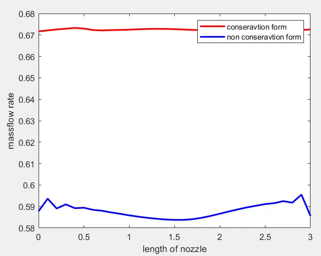
Figure 11
since the back pressure in this case is zero the massflow rate is constant along the length of the nozzle (ideally it shloud be a horizontal line but becauses of numerical approximations error are introduced so it deviates from the ideal solution). the conservation form gives closer approximation to the ideal solution comapred to that of non-conservation form.the below plot is generated for 31 grid points
GRID INDEPENDENCE TEST RESULTS
CONSERVATION FORM TABLE
primitive variables are taken at throat section
| NO OF GRID POINTS | DENSITY | TEMPERATURE | PRESSURE | MASSFLOW RATE | TIME(SEC) |
| 31 | 0.7092 | 0.7941 | 0.5632 | 0.6727 | 594 |
| 61 | 0.7088 | 0.7969 | 0.5649 | 0.6683 | 596 |
| 91 | 0.707 | 0.7965 | 0.5631 | 0.6647 | 614 |
NON CONSERVATION FORM TABLE
primitive variables are taken at throat section
| NO OF GRID POINTS | DENSITY | TEMPERATURE | PRESSURE | MASSFLOW RATE | TIME (SEC) |
| 31 | 0.6387 | 0.8365 | 0.5342 | 0.5838 | 675 |
| 61 | 0.6377 | 0.8345 | 0.5327 | 0.5827 | 607 |
| 91 | 0.6404 | 0.8368 | 0.5359 | 0.5874 | 558 |
CONCLUSIONS
It is clear form the above data that by increasing no of grid points there is an insignificant change in the primitive variables estimation in both conservation and non conseravtion form.the time taken for estimation in conseravtion form is increasing with increase in grid points whereas in non conservation form decreases with increase in grid points
with 31 grid points numerical estimation of massflow rate in conservation form is more accurate comparied to that of non conservation form. but the estimation of primitive variables is in non conservation form is more smooth and accurate comparied to that of conservation form.as the no of grid point increases the massflow rate estimation comes first closer to accurate solution but after further increase in grid point have deviated the estimation
with 61 grid points the numerical estimation of massflow rate even more accurate in conservation form comparied to that of non conservation form