Solving the steady and unsteady 2D heat conduction problem
INTRODUCTION
Conduction takes place in all phases: solid, liquid, and gas .In Solids, conduction is mediated by the combination of vibrations and collisions of molecules, of propagation and collisions of phonons, and of diffusion and collisions of free electrons. In gases and liquids, conduction is due to the collisions and diffusion of molecules during their random motion. The law of heat conduction, also known as Fourier's law, states that the rate of heat transfer through a material is proportional to the negative gradient in the temperature and to the area, at right angles to that gradient, through which the heat flows.
`q=-k * Delta t`
q is the local heat flux density,`W*overset (-2)(m)`
k is the material conductivity,`W*overset (-1)(m)*overset (-1)(k)`
`Delta t` is the temperature gradient,`K*overset(-1)(m)`
Fourier law in differential form
`frac{partial T}{partial t}=alpha(frac{partialT}{partial x^2 }+frac{partialT}{partial y^2 }+frac{partialT}{partial z^2 })`
Steady-state conduction is the form of conduction that happens when the temperature difference driving the conduction are constant, so that the spatial distribution of temperatures in the conducting object does not change any further.
During any period in which temperatures changes in time at any place within an object, the mode of thermal energy flow is termed transient conduction.
Steady state heat conduction and Transient conduction's Finite Difference Method equation can be solved with the help of (i)Implicit Schemes (ii)Explicit Schemes
Derivation
(i)Implicit Scheme
Works with Unknown time step or new time step values on the Finite difference method
For steady state heat conduction
`frac{partial T}{partial x^2}+frac{partial T}{partial y^2}=0` ----- 1 eq
`f(x+a)=f(x)+frac{f'(x)*dx}{1!}+frac{f''(x)*dx^2}{2!}+....`
`f(x-a)=f(x)-frac{f'(x)*dx}{1!}+frac{f''(x)*dx}{2!}+....`
Add f(x+a) & f(x-a)
`f''(x)=frac{f(x+a)+f(x-a)-2*f(x)}{dx^2}`
Substuting f''(x) in 1eq
`frac{T(i,j-1)+T(i,j+1)-2*T(i,j)}{partial x^2}+frac{T(i-1,j)+T(i+1,j)-2*T(i,j)}{partial y^2}=0`
`T(i,j)=frac{1}{frac{2*(partial x^2+partial y^2)}{partial x^2*partial y^2}}*(frac{T(i,j-1)+T(i,j+1)}{partial x^2}+frac{T(i-1,j)+T(i+1,j)}{partial y^2})`
For Transient heat conduction
`frac{partial T}{partial t}=alpha*(frac{partial ^2T}{partial x^2}+frac{partial ^2T}{partial y^2})`
Substituting f''(x) in above equation
`frac{T^(n+1)-T^n}{Delta t}=alpha*(frac{T(i,j-1)+T(i,j+1)-2*T(i,j)}{Delta x^2}+frac{T(i-1,j)+T(i+1,j)-2*T(i,j)}{Delta y^2})^(n+1))`
`T(i,j)^(n+1)*(1+frac{alpha*partial t}{Delta x^2}+frac{alpha*partial t}{Delta y^2})=T(i,j)^n+frac{alpha*partial T}{Delta x^2}*(T(i,j-1)+T(i,j+1))^(n+1)+frac{alpha*partial T}{Delta y^2}*(T(i-1,j)+T(i+1,j))^(n+1)`
`T(i,j)^(n+1)=frac{T(i,j)^n}{(1+frac{alpha*partial t}{Delta x^2}+frac{alpha*partial t}{Delta y^2})}+frac{alpha*partial T}{Delta x^2 * (1+frac{alpha*partial t}{Delta x^2}+frac{alpha*partial t}{Delta y^2})}*(T(i,j-1)+T(i,j+1))^(n+1)+frac{alpha*partial T}{Delta y^2 * (1+frac{alpha*partial t}{Delta x^2}+frac{alpha*partial t}{Delta y^2})}*(T(i-1,j)+T(i+1,j))^(n+1)`
Implicit schemes are solved using Jacobi,Guass-siedel,SOR(Sucessive Over-Relaxation) method
Jacobi Method-In numerical linear algebra, the Jacobi is an iterative algorithm for determining the solutions of a strictly diagonally dominant system of linear equations. Each diagonal element is solved for, and an approximate value is plugged in. The process is then iterated until it converges.
Guass-Siedel Method-Though it can be applied to any matrix with non-zero elements on the diagonals, convergence is only guaranteed if the matrix is either strictly diagonally dominant,or symmetric and positive definite. The computation of `x^(k+1)` uses the elements of `x^(k+1)` that have already been computed, and only the elements of `x^(k)` that have not been computed in the k+1 iteration
Sucessive Over relaxation method(SOR)-In numerical linear algebra, the method of successive over-relaxation (SOR) is a variant of the Gauss–Seidel method for solving a linear system of equations, resulting in faster convergence.proved that if A is symmetric and positive-definite then the successive relaxation factor should be inbetween 0 to 2. Values of factor is > 1 are used to speed up convergence of a slow-converging process, while values of factor <1 are often used to help establish convergence of a diverging iterative process or speed up the convergence of an overshooting process..
ii.Explict scheme
Steady state heat conduction
Works with known time steps in the Finite Difference Method
`T(i,j)=frac{1}{frac{2*(partial x^2+partial y^2)}{partial x^2*partial y^2}}*(frac{T(i,j-1)+T(i,j+1)}{partial x^2}+frac{T(i-1,j)+T(i+1,j)}{partial y^2})`
Transient Heat Conduction
`T(i,j)^(n+1)=T(i,j)^n*(1-frac{alpha*partial t}{Delta x^2}-frac{alpha*partial t}{Delta y^2})+frac{alpha*partial T}{Delta x^2 }*(T(i,j-1)+T(i,j+1))^(n)+frac{alpha*partial T}{Delta y^2 }*(T(i-1,j)+T(i+1,j))^(n)`
Main program
(i)Unsteady state
Implicit Method
clear all
close all
clc

%input
L=1;
nx=20;
ny=20;
dt=0.1;
alpha=1.4;  %thermal diffusivity
error=9e+9;
x=linspace(0,L,nx)
y=linspace(0,L,ny)
dx=x(2)-x(1)
dy=y(2)-y(1)
[xx yy]=meshgrid(x,y)
T(1:nx,1:ny)=298;
% Temperature in kelvins
T(1,1:ny)=600  %Temperature at Top
T(nx,1:ny)=900 %Temperature at Bottom
T(1:nx,1)=400  %Temperature at left
T(1:nx,ny)=800 %Temperature at Right

T(1,1)=(400+600)/2 %Temperature at Left-Top corner
T(1,ny)=(800+600)/2  %Temperature at right-top corner
T(nx,1)=(900+400)/2  %Temperature at bottom-left corner
T(nx,ny)=(900+800)/2 %Temperature at bottom-right corner
tol=1e-4;
t=T;
T_j=T;
T_SOR=T;
T_G1=T;
 T_old_timestep=T;
 Jacobi_iter=0;
 time=0
%Jacobi method
tic
for time_J=1:dt:200
    while error>tol
        for i=2:1:nx-1
            for j=2:1:ny-1

                k1=(alpha * dt)/(dx^2)
                k2=(alpha * dt)/(dy^2)
                term1=1/(1+(2*k1)+(2*k2))
               T_j(i,j)=(term1*T_old_timestep(i,j))+((k1*term1)*(t(i,j+1)+t(i,j-1)))+((k2*term1)*(t(i-1,j)+t(i+1,j)));
            end
        end
        error=max(max(abs(t-T_j)))
        t=T_j;
        Jacobi_iter=Jacobi_iter+1;
    end
error1=max(max(abs(T_old_timestep-T_j)))
    T_old_timestep=T_j;
   error=9e+9;
   if error1tol
        for i=2:1:nx-1
            for j=2:1:ny-1

                k1=(alpha * dt)/(dx^2)
                k2=(alpha * dt)/(dy^2)
                term1=1/(1+(2*k1)+(2*k2))
               T_G(i,j)=(term1*T_old_timestep(i,j))+((k1*term1)*(t(i,j+1)+T_G(i,j-1)))+((k2*term1)*(T_G(i-1,j)+t(i+1,j)));
            end
        end
        error=max(max(abs(t-T_G)));
        t=T_G;
        Guass_iter=Guass_iter+1;
    end

    error1=max(max(abs(T_old_timestep-T_G)))
    T_old_timestep=T_G;
    error=9e+9;
    if error1tol
        for i=2:1:nx-1
            for j=2:1:ny-1

                k1=(alpha * dt)/(dx^2)
                k2=(alpha * dt)/(dy^2)
                term1=1/(1+(2*k1)+(2*k2))
               T_G1(i,j)=(term1*T_old_timestep(i,j))+((k1*term1)*(t(i,j+1)+T_SOR(i,j-1)))+((k2*term1)*(T_SOR(i-1,j)+t(i+1,j)));
               T_SOR(i,j)=(t(i,j)*(1-alpha1))+(T_G1(i,j)*alpha1)
            end
        end
        error=max(max(abs(t-T_SOR)))
        t=T_SOR;
        SOR_iter=SOR_iter+1;
    end
     error1=max(max(abs(T_old_timestep-T_SOR)))
  T_old_timestep=T_SOR;
    error=9e+9;
    if error1
Plots
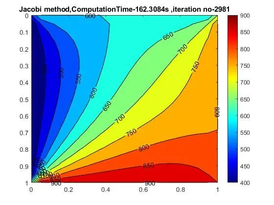
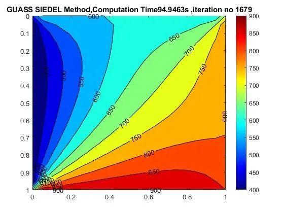
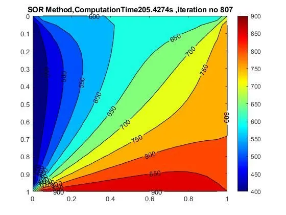
Explicit Scheme program
clc
clear all
close all


L=1;
nx=20;
ny=20;
dt=0.0001;
alpha=1.4;
error=9e+9;;
x=linspace(0,L,nx)
y=linspace(0,L,ny)
dx=x(2)-x(1)
dy=y(2)-y(1)
[xx yy]=meshgrid(x,y)
T(1:nx,1:ny)=300;
% Temperature in kelvins
T(1,1:ny)=600  %Temperature at Top
T(nx,1:ny)=900 %Temperature at Bottom
T(1:nx,1)=400  %Temperature at left
T(1:nx,ny)=800 %Temperature at Right

T(1,1)=(400+600)/2 %Temperature at Left-Top corner
T(1,ny)=(800+600)/2  %Temperature at right-top corner
T(nx,1)=(900+400)/2  %Temperature at bottom-left corner
T(nx,ny)=(900+800)/2 %Temperature at bottom-right corner
tol=1e-4;
t=T;
T_j=T;
T_SOR=T;
T_G1=T;
 T_new_timestep=T;
 iter_no=0;

 tic
for time=1:dt:200
    for i=2:1:nx-1
        for j=2:1:ny-1
            k1=(alpha * dt)/ (dx^2)
            k2=(alpha * dt)/ (dy^2)
            T_new_timestep(i,j)=(t(i,j)*(1-(2*k1)-(2*k2)))+(k1*(t(i,j-1)+t(i,j+1)))+(k2*(t(i-1,j)+t(i+1,j)));
        end
    end
    error=max(max(abs(T_new_timestep-t)))
    t=T_new_timestep;
   if error
Plots
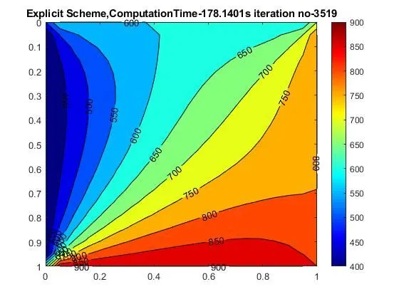
(ii) Steady state Program
clear all
close all
clc

%input
L=1;
nx=20;
ny=20;
dt=0.1;
alpha=1.4;  %Thermal Diffusivity
error=9e+9;;
x=linspace(0,L,nx)
y=linspace(0,L,ny)
dx=x(2)-x(1)
dy=y(2)-y(1)
[xx yy]=meshgrid(x,y)
T(1:nx,1:ny)=298;
% Temperature in kelvins
T(1,1:ny)=600  %Temperature at Top
T(nx,1:ny)=900 %Temperature at Bottom
T(1:nx,1)=400  %Temperature at left
T(1:nx,ny)=800 %Temperature at Right

T(1,1)=(400+600)/2 %Temperature at Left-Top corner
T(1,ny)=(800+600)/2  %Temperature at right-top corner
T(nx,1)=(900+400)/2  %Temperature at bottom-left corner
T(nx,ny)=(900+800)/2 %Temperature at bottom-right corner
tol=1e-4;
t=T;
T_j=T;
T_SOR=T;
T_G1=T;
 T_new_timestep=T;
 Jacobi_iter=0;
 time=0
%Jacobi method
tic
    while error>tol
        for i=2:1:nx-1
            for j=2:1:ny-1

                k1=(1)/(dx^2)
                k2=(1)/(dy^2)
                term1=1/(2*(k1+k2))
               T_j(i,j)=(term1*(k1*(t(i,j+1)+t(i,j-1))))+((k2*term1)*(t(i-1,j)+t(i+1,j)));
            end
        end
        error=max(max(abs(t-T_j)))
        t=T_j;
        Jacobi_iter=Jacobi_iter+1;
    end
Time=toc
 figure(1)
    [M,N]=contourf(xx,yy,T_j);
    title(['Jacobi iteration ,Computation Time-',num2str(Time),'s iteration no-',num2str(Jacobi_iter)]);
    set(gca,'YDIR','reverse')
    clabel(M,N)
    colormap(jet)
    colorbar


%Guass siedel method
t=T
T_G=T
T_new_timestep=T
Guass_iter=0
error=9e+9;
error1=9e+9
time=0
tic
    while error>tol
        for i=2:1:nx-1
            for j=2:1:ny-1
               k1=(1)/(dx^2)
                k2=(1)/(dy^2)
                term1=1/(2*(k1+k2))
               T_G(i,j)=(term1*(k1*(t(i,j+1)+T_G(i,j-1))))+((k2*term1)*(T_G(i-1,j)+t(i+1,j)));;
            end
        end
        error=max(max(abs(t-T_G)));
        t=T_G;
        Guass_iter=Guass_iter+1;
    end

Time=toc
 figure(2)
    [M,N]=contourf(xx,yy,T_G);
    title(['Guass iteration, computationTime-',num2str(Time),'s , iteration no ',num2str(Guass_iter)]);
    set(gca,'YDIR','reverse')
    clabel(M,N)
    colormap(jet)
    colorbar

%SOR Method
t=T
T_new_timestep=T
SOR_iter=0
alpha1=1.4
error=9e+9
tic
    while error>tol
        for i=2:1:nx-1
            for j=2:1:ny-1

                 k1=(1)/(dx^2)
                k2=(1)/(dy^2)
                term1=1/(2*(k1+k2))
               T_G1(i,j)=(term1*(k1*(t(i,j+1)+T_G1(i,j-1))))+((k2*term1)*(T_G1(i-1,j)+t(i+1,j)));
               T_SOR(i,j)=(t(i,j)*(1-alpha1))+(T_G1(i,j)*alpha1)
            end
        end
        error=max(max(abs(t-T_SOR)))
        t=T_SOR;
        SOR_iter=SOR_iter+1;
    end

 Time=toc

figure(3)
    [M,N]=contourf(xx,yy,T_SOR);
  title(['SOR iteration,ComputationTime-',num2str(Time),'s ,iteration no ',num2str(SOR_iter)]);
    set(gca,'YDIR','reverse')
    clabel(M,N)
    colormap(jet)
    colorbar
Plots
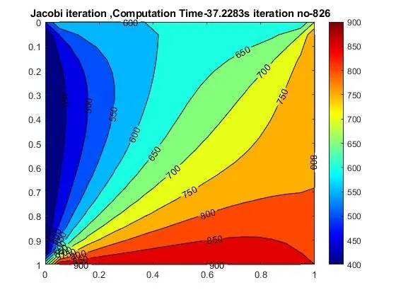
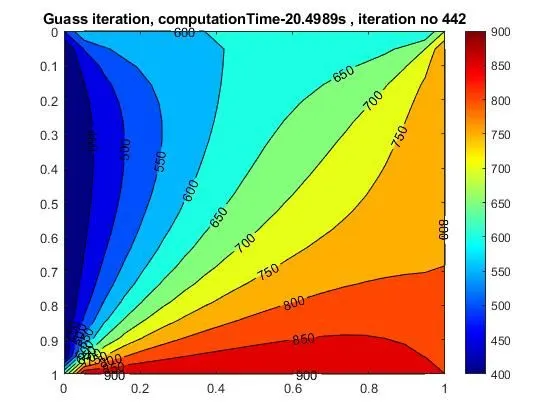
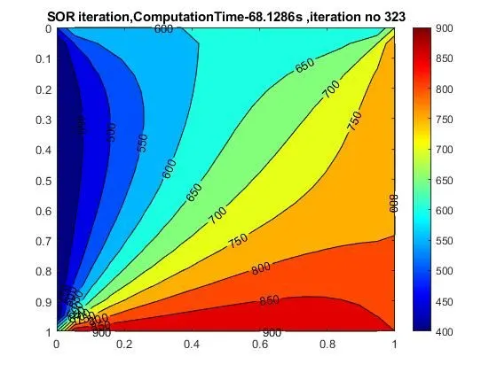
Conclusion
It clearly shows that ,implicit schemes can be carryout for change in time is large, with minimum number of iterations were as for explicit scheme need a change in time is small to satisfy a CFL condition
CFL condition= `frac{alpha *dt }{dx^2}+frac{alpha *dt }{dy^2}<0.5`
If CFL value near to the 0.5 then the iteration get reduced
From implicit scheme, We can compute with Minimum no of iterations by using SOR method (Guass Siedel).