Week 5.1 - Mid term project - Solving the steady and unsteady 2D heat conduction problem
Aim:
The aim of this code is to solve the 2D heat conduction equation for a steady-state scenario using iterative solvers: Jacobi, Gauss-Seidel, and Successive Over-Relaxation (SOR). The solution is visualized using contour plots to show the steady-state temperature distribution within the domain.
Theory:
Theory-
Conduction is a mode of heat transfer, that generally takes place in solids due to temperature differences associated with free electron and lattice vibration.
A generalized conduction equation is given
Thermal diffusivity is a thermophysical property of a material defined as the ratio of the thermal conductivity of the material to its thermal capacity.
Since the problem is 2D and there is no heat generation considered, those terms are neglected. So the equation represents unsteady 2D heat conduction (parabolic).
A steady-state does not take the time derivative into account. The 2D steady state heat conduction problem is thus given by rewriting it as follows:
Difference equations for the steady-state and unsteady-state 2D conduction equations are derived to obtain the numerical solution.
Steady-state 2d heat conduction equation
Transient Heat conduction equation in implicit form
Transient Heat conduction equation in explicit form
Now, using the iterative solvers, we will run the code and solve the above equation.
Steady State Analysis of a 2d Heat Conduction
- The first inputs are defined into variables, and the temperature array is created.
- Boundary conditions are introduced into the temperature array, and at corners, boundary values are averaged.
- Constants like alpha, omega, and tolerance are defined to run the iteration.
- Input must be provided by the user, to choose the iterative method.
- The if-else loop is used to solve the equation using the selected (input from the user) iterative technique.
- Iterative techniques are run using a while loop until the desired accuracy is attained.
- At each iterative step, the temperature values at each node are computed using two for loops.
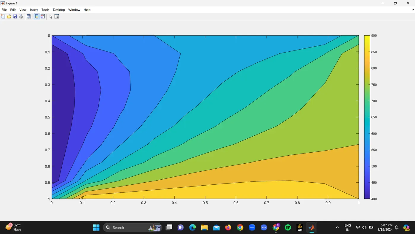
- Using the 'conturf' command, the temperature distribution graph is finally produced.
Method of Jacobi iterations:
T(i,j)=1k[T(i−1,j)+T(i+1,j)△x2+T(i,j−1)+T(i,j+1)△y2�(�,�)=1�[�(�-1,�)+�(�+1,�)△�2+�(�,�-1)+�(�,�+1)△�2
Gauss-Seidel Iterations method
T(i,j)=1k[T(i−1,j)+Told(i+1,j)△x2+T(i,j−1)+Told(i,j+1)△y2]�(�,�)=1�[�(�-1,�)+����(�+1,�)△�2+�(�,�-1)+����(�,�+1)△�2]
SOR iterations method:
T(i,j)=((1-w)Told+omega)1/k[(T(i-1,j)+Told(i+1,j))/(trianglex^2)+(T(i,j-1)+Told(i,j+1))/(triangley^2)]
conditions for omega(w)= w>1 = over relaxation
w<1 = under relaxation
w= 1.1,1.2 = perfect solution
Procedure:
1. Initialization: The code starts by clearing the workspace, closing all figures, and clearing the command window. It then sets up the domain and discretization parameters, including the number of nodes and the domain length.
2. Grid Setup: The code defines the grid points in the x and y directions using `linspace` and calculates the grid spacing `dx` and `dy`.
3. Initial Temperature Distribution: An initial temperature distribution is set for all nodes within the domain, with a default value of 300 K. Boundary conditions are applied at the left, right, bottom, and top of the domain, with specific values provided.
4. Iterative Solvers: The code implements three iterative solvers: Jacobi, Gauss-Seidel, and SOR. Each solver iterates over the grid points, updating the temperature at each point based on the heat conduction equation and the chosen method. The solvers differ in how they update the temperature values at each iteration.
Jacobi Method: Updates the temperature at each grid point based on the average of the temperatures at the neighboring points.
The Gauss-Seidel Method: is similar to Jacobi but uses the updated temperature values from the current iteration for the calculation of the next iteration.
SOR Method: Uses an over-relaxation factor to accelerate convergence. The temperature at each grid point is updated based on a weighted average of the current and updated temperatures.
5. Convergence Criteria: The code checks for convergence by comparing the maximum absolute difference between the old and new temperature distributions. The iteration continues until the difference is less than a specified tolerance.
6. Visualization: After convergence, the code visualizes the steady-state temperature distribution using a contour plot. The plot is generated using `meshgrid` to create a grid of x and y values, which are then used with `contourf` to create the contour plot.
The choice of iterative solver can significantly affect the convergence rate and the accuracy of the solution. The SOR method, with its over-relaxation factor, generally converges faster than the Jacobi and Gauss-Seidel methods.
The boundary conditions play a crucial role in determining the solution. Incorrect or inadequate boundary conditions can lead to inaccurate results.
The visualization of the temperature distribution provides insights into the heat conduction pattern within the domain, which can be useful for understanding the physical phenomena being modeled.
Conclusion:
This code effectively demonstrates the application of iterative solvers to solve the 2D heat conduction equation for a steady-state scenario. The choice of solver and the accuracy of the solution depend on the specifics of the problem and the boundary conditions. The visualization of the temperature distribution provides valuable insights into the heat conduction pattern within the domain.
Code:
STEADY STATE ANALYSIS:
clear all
close all
clc

% Domain and discretization parameters
numNodes = 10;
domainLength = 1;

% Grid points
x = linspace(0, domainLength, numNodes);
y = linspace(0, domainLength, numNodes);
dx = domainLength / (numNodes - 1);
dy = domainLength / (numNodes - 1);

% Initial temperature distribution
T = 300 * ones(numNodes, numNodes);

% Boundary conditions
T(1:end, 1) = 400;
T(1:end, end) = 800;
T(end, 1:end) = 900;
T(1, 1:end) = 600;
T(1, 1) = 500;
T(end, 1) = 650;
T(1, end) = 700;
T(end, end) = 850;

% Copy of temperature for iteration
T_old = T;

% Constants
K = (2 * (dx^2 + dy^2)) / (dx^2 * dy^2);
omega = 1.2;

% Error and tolerance
error = 10;
tol = 1e-4;
iterations = 0;

% Method selection
method = input('Enter 1 for Jacobi, 2 for Gauss-Seidel, 3 for SOR: ');

% Iterative solver loop
while error > tol
    for i = 2:numNodes-1
        for j = 2:numNodes-1
            if method == 1 % Jacobi
                T(i, j) = (T_old(i+1, j) + T_old(i-1, j) + T_old(i, j+1) + T_old(i, j-1)) / 4;
            elseif method == 2 % Gauss-Seidel
                T(i, j) = (T(i+1, j) + T(i-1, j) + T(i, j+1) + T(i, j-1)) / 4;
            elseif method == 3 % SOR
                T(i, j) = (1 - omega) * T_old(i, j) + (omega / 4) * (T_old(i+1, j) + T_old(i-1, j) + T_old(i, j+1) + T_old(i, j-1));
            end
        end
    end
    error = max(max(abs(T_old - T)));
    T_old = T;
    iterations = iterations + 1;
end

% Visualization
[X, Y] = meshgrid(x, y);
contourf(X, Y, T);
colorbar;
set(gca, 'ydir', 'reverse');
Command Window :
Enter 1 for Jacobi, 2 for Gauss-Seidel, 3 for SOR: 1
>> iterations

iterations =

   207

>>
Plot:
CODE:
UNSTEADY-STATE ANALYSIS:
clear all; close all; clc;

% Domain and discretization parameters
numNodes = 10;
domainLength = 1;

% Grid points
x = linspace(0, domainLength, numNodes);
y = linspace(0, domainLength, numNodes);
dx = domainLength / (numNodes - 1);
dy = domainLength / (numNodes - 1);
dt = 1/10;

% Initial temperature distribution
T = 300 * ones(numNodes, numNodes);

% Boundary conditions
T(1:end, 1) = 400;
T(1:end, end) = 800;
T(end, 1:end) = 900;
T(1, 1:end) = 600;
T(1, 1) = 500;
T(end, 1) = 650;
T(1, end) = 700;
T(end, end) = 850;

% Copy of temperature for iteration
T_old = T;
T_prev = T;

% Constants
alpha = 1.5;
omega = 1.15;
K1 = (alpha * dt) / (dx^2);
K2 = (alpha * dt) / (dy^2);

% Method selection
approach = input('Enter 1 for implicit or Enter 2 for explicit: ');
method = input('Enter 1 for Jacobi, 2 for Gauss-Seidel, 3 for SOR: ');

% Iterative solver loop
for nt = 1:1500
    error = 10;
    tol = 1e-4;
    while error > tol
        for i = 2:numNodes-1
            for j = 2:numNodes-1
                if approach == 1 % Implicit methods
                    term1 = 1 / (1 + (2 * K1) + (2 * K2));
                    term2 = K1 * (T_old(i+1, j) + T_old(i-1, j));
                    term3 = K2 * (T_old(i, j+1) + T_old(i, j-1));
                    if method == 1 % Jacobi
                        T(i, j) = term1 * (T_prev(i, j) + term2 + term3);
                    elseif method == 2 % Gauss-Seidel
                        T(i, j) = term1 * (T(i, j) + term2 + term3);
                    else % SOR
                        T(i, j) = (1 - omega) * T_old(i, j) + (omega * term1 * (T_prev(i, j) + term2 + term3));
                    end
                else % Explicit method
                    term1 = K1 * (T_prev(i+1, j) - 2 * T_prev(i, j) + T_prev(i-1, j));
                    term2 = K2 * (T_prev(i, j+1) - 2 * T_prev(i, j) + T_prev(i, j-1));
                    T(i, j) = T_prev(i, j) + term1 + term2;
                end
            end
        end
        error = max(max(abs(T_old - T)));
        T_old = T;
        T_prev = T;
    end
end

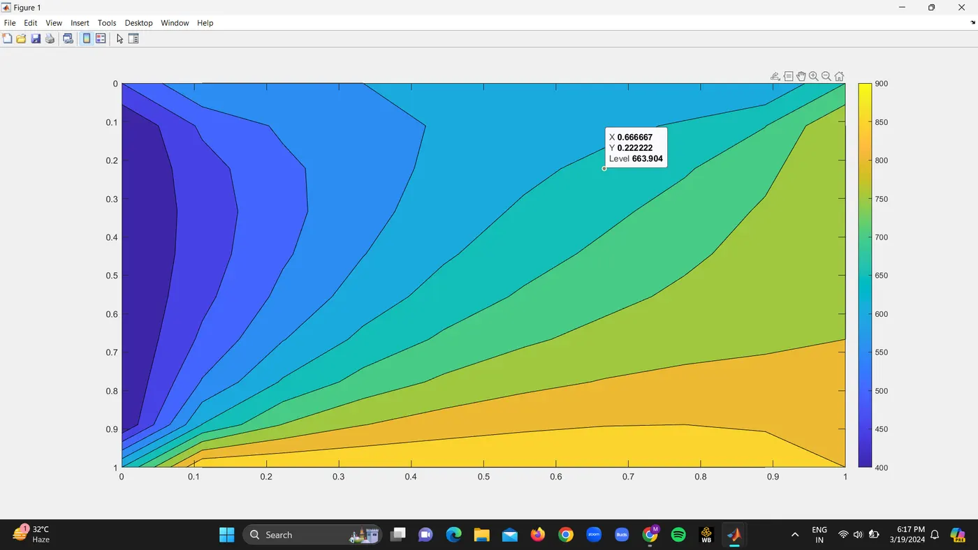
% Visualization
[X, Y] = meshgrid(x, y);
figure(1);
contourf(X, Y, T);
colorbar;
set(gca, 'ydir', 'reverse');
COMMAND WINDOW:
>> T

T =

  500.0000  600.0000  600.0000  600.0000  600.0000  600.0000  600.0000  600.0000  600.0000  700.0000
  400.0000  509.5965  558.3269  585.5626  604.0876  619.2937  635.0648  657.0610  698.6291  800.0000
  400.0000  480.0591  538.1484  579.8361  611.4939  638.0225  663.9044  694.5502  737.4553  800.0000
  400.0000  472.4913  534.3717  584.1394  624.0296  657.3978  687.9801  719.7802  756.6418  800.0000
  400.0000  475.5345  542.7076  598.3202  643.0875  679.5589  710.8380  739.9488  769.3317  800.0000
  400.0000  486.9391  562.6040  623.3463  670.4411  706.9125  735.8641  759.8451  780.7363  800.0000
  400.0000  509.6179  597.4229  662.0199  708.4180  741.7861  765.8606  782.8314  793.7684  800.0000
  400.0000  554.1097  655.4498  718.8925  759.4248  785.9533  802.9608  811.8516  811.5059  800.0000
  400.0000  651.3709  751.3741  798.6755  824.4355  839.6416  848.1776  850.1082  840.4035  800.0000
  650.0000  900.0000  900.0000  900.0000  900.0000  900.0000  900.0000  900.0000  900.0000  850.0000

>>
PLOT:
Observations:
- 1. The temperature distribution plot obtained for both the steady and unsteady conditions is the same.
- Because in transient analysis, the solution approaches steady-state.
- 2. The top, bottom, left, and right sides of the graphs represent their respective boundary conditions.