Week 5.1 - Mid term project - Solving the steady and unsteady 2D heat conduction problem
Objective:
Solve the 2D heat conduction equation by using the point iterative techniques
1.Jacobi
2.Gauss-seidel
3.Successive over-relaxiation
Absolute error criteria is le-4
1.Steady state analysis
2.Transient state analysis using explict and implicit schemes.
Description:
The general heat conduction equation with no heat generation is
`∂ T/ ∂ t = ∝ ( ∂ ^2 T/ ∂ x ^2 + ∂ ^2 T/ ∂ y ^2 + ∂ ^2 T /∂ z ^2 )`
where T is the temperature and α is the thermal diffusivity and (x,y,z,t) are space and time variables respectively.
The 2D stedy state heat conduction equation with no heat generation is
`(∂ ^2 T )/(∂ x ^2 )+ (∂ ^2 T) /(∂ y ^2)=0`
The 2D transient state heat conduction equation with no heat generation is
`(∂ T/ ∂ t) = ∝ (( ∂ ^2 T)/ (∂ x ^2 )+ (∂ ^2 T )/(∂ y ^2 ))`
Descritization:
We will use the central differencing method to discretize our second-order partial differential equation of T w.r.t x and y because it is elliptical or we can say it takes information from all direction in the mesh and will use Forward differenciing method to discritize our time derivative term of T w.r.t t as it is hyperbolic or we can say it takes information from left to right.
Let Ti,jL be the temperature at the point of intersection of ith row and jth column in the assumed square field. The above PDE can be discretized as follows
`(∂ ^2 T)/( ∂ x^ 2)= (T_ (i − 1 , j )− 2 ⋅ T _i ,_j + T _(i + 1, j))/( Δ x 2)`
`(∂^ 2 T) /(∂ y^ 2) =( T_ (i − 1 , j )− 2 ⋅ T_ (i , j )+ T_ (i + 1 , j ))/(Δ y^ 2)`
`(∂^ 2 T) /(∂ y^ 2) =(T_(i,j)^(n+1)-T_(i,j)^n)/(Δt)`
Descritization from of steady state conduction is
`(∂^ 2 T)/ (∂ x^ 2) + (∂ ^2 T)/( ∂ y ^2) = 0`
`(T_(i-1,j)-2.T_i,_j+T_(i+1,j ))/(Δx^2)+(T_(i,j-1)-2.T_i,_j+T_(i,j +1))/(Δy^2)`
By further simplification we can get
`T_i,_j=(1/k)((T_(i-1,j)+T_(i+1,j) )/(Δx^2)+(T_(i,j-1)+T_(i,j +1))/(Δy^2))`
where
`k=2((Δx^2+Δy^2)/(Δx^2.Δy^2))`
Thus above equation gives the temperature values at each node as a function of the temperature of its neighbouring nodes.
The above equation for temperature distribution will be solved using the fixed point method with the help of iterative solvers like jocobi, gauss-siedel and successive over relaxation(SOR) to study the comparison among these iterative solvers.
Jacobi iterative solver:
In jacobi method, each iteration is done using a set of previous values, even if new values are available in the middle of an iteration. Like when we are solving n+1 iteration and for i the node we will use the values of previous (n) iteration even if we have to update values of nodes in current iteration. So this method is called method of simultaneous displacements.
The 2D stedy state heat conduction eqution for this method is
`T_i,_j=(1/k)((T_(i-1,j)^n+T_(i+1,j)^n)/(Δx^2)+(T_(i,j-1)^n+T_(i,j+1)^n)/(Δy^2))`
Gauss-seidel method
In Gauss-Seidel, as soon as you find a new value in the current iteration you will use it for finding other values in the current iteration.
like when we are solving for n+1 iteration and for i the node will use all the available values up to i-1 nodes of current iteration(n+1) and use i+1 node values and above values of previous iteration(n). So we get more converged values. In this method is called method of spontaneous displacements.
The 2D steady state heat conduction equation for this method is
`T_i,_j=(1/k)((T_(i-1,j)^(n+1)+T_(i+1,j)^(n+1))/(Δx^2)+(T_(i,j-1)^(n+1)+T_(i,j+1)^(n+1))/(Δy^2))`
Successive Over-Relaxiation(SOR)method:
It is a variant of Gauss-Sidel method for solving a linear system of equations, resulting in faster convergence. You can also use jacobi method. Here an extra term called relaxation factor (omega) is multiplied to gauss seidel generated term to scale the convergence rate and solve the equation faster. To calculate new value we take old value and take a parameter omega and take rate of change.
The 2D steady state heat conduction equation for this method is
For scaling jacobian method, where Tj is the result of jacobian method.
Tn+1i,j=Tni,j T(1-α)+α/k(Tjac or Tguass)
Code:
%Using iterative technique solve the 2D heat conduction
%jacobi method
clear all
close all
clc
l=1; % Length of the domain
nx=10;%define number of grid points in x_axis
ny=nx;%defines number of grid points in y_axis
x=linspace(0,1,nx);
y=linspace(0,1,ny);
dx=l/(nx-1);%grid spacing
dy=l/(ny-1);%grid spacing
k=2*((dx^2+dy^2)/(dx^2*dy^2));% Coefficient for gauss-seidel method
% Define boundary conditions
top=600;
bottom=900;
left=400;
right=800;
% Initialize temperature matrix
T=ones(nx,ny);
T(1,:)=top;
T(ny,:)=bottom;
T(:,1)=left;
T(:,nx)=right;

T(1,1)=(top+left)/2;
T(1,nx)=(top+right)/2
T(ny,1)=(bottom+left)/2;
T(ny,nx)=(right+bottom)/2

told=T;% Initialize the previous temperature matrix
tnew=T;
error=9e9;
tol=1e-4;
iterative_solvers=1;
tic
if iterative_solvers==1;
    jacobi_iterator=1
    while (error>tol);
        for i=2:nx-1;
            for j=2:ny-1;
                % Update temperature using jacobi iteration formula
                T(i,j)=(1/k)*((told(i+1,j)+told(i-1,j))/(dx^2)+(told(i,j+1)+told(i,j-1))/(dy^2));
            end
        end
        % Calculate the maximum absolute difference between old and new temperature matrices
        error=max(max(abs(told-T)));
        told=T;% Update the old temperature matrix for the next iteration
        time_required=toc% Calculate the elapsed time
        jacobi_iterator=jacobi_iterator+1;
        % Display the current temperature distribution
        contourf(x,flip(y),T)
        colorbar
        xlabel('x Domain')
        ylabel('Y Domain')
        title_text=sprintf('2D heat conduction jacobi iterator=%d;computation time:%0.3f s',jacobi_iterator,time_required);
        title(title_text)
        pause(0.03)
    end
end
%Using iterative technique solve the 2D heat conduction
%Gauss-seidel method
clear all
close all
clc
l=1; % Length of the domain
nx=10;%define number of grid points in x_axis
ny=nx;%defines number of grid points in y_axis
x=linspace(0,1,nx);
y=linspace(0,1,ny);
dx=l/(nx-1);%grid spacing
dy=l/(ny-1);%grid spacing
k=2*((dx^2+dy^2)/(dx^2*dy^2));% Coefficient for gauss-seidel method
% Define boundary conditions
top=600;
bottom=900;
left=400;
right=800;
% Initialize temperature matrix
T=ones(nx,ny);
T(1,:)=top;
T(ny,:)=bottom;
T(:,1)=left;
T(:,nx)=right;
T(1,1)=(top+left)/2;
T(1,nx)=(top+right)/2
T(ny,1)=(bottom+left)/2;
T(ny,nx)=(right+bottom)/2
told=T;% Initialize the previous temperature matrix
tnew=T;
error=9e9;
tol=1e-4;
iterative_solvers=1;
tic
if iterative_solvers==1;
gs_iterator=1
while (error>tol);
for i=2:nx-1;
for j=2:ny-1;
% Update temperature using gauss-seidel iteration formula
T(i,j)=(1/k)*((told(i+1,j)+T(i-1,j))/(dx^2)+(told(i,j+1)+T(i,j-1))/(dy^2));
end
end
% Calculate the maximum absolute difference between old and new temperature matrices
error=max(max(abs(told-T)));
told=T;% Update the old temperature matrix for the next iteration
time_required=toc% Calculate the elapsed time
gs_iterator=gs_iterator+1;
% Display the current temperature distribution
contourf(x,flip(y),T)
colorbar
xlabel('x Domain')
ylabel('Y Domain')
title_text=sprintf('2D heat conduction Gauss-seidel iterator=%d;computation time:%0.3f s',gs_iterator,time_required);
title(title_text)
pause(0.03)
end
end%Using iterative technique solve the 2D heat conduction
%succesive-over relaxiation
clear all
close all
clc
l=1;% Length of the domain
nx=10;%define number of grid points in x_axis
ny=nx;%defines number of grid points in y_axis
x=linspace(0,1,nx);
y=linspace(0,1,ny);
dx=l/(nx-1);%grid spacing
dy=l/(ny-1);%grid spacing
k=2*((dx^2+dy^2)/(dx^2*dy^2));
% Define boundary conditions
top=600;
bottom=900;
left=400;
right=800;
% Initialize temperature matrix
T=ones(nx,ny);
T(1,:)=top;
T(ny,:)=bottom;
T(:,1)=left;
T(:,nx)=right;
T(1,1)=(top+left)/2;
T(1,nx)=(top+right)/2;
T(ny,1)=(bottom+left)/2;
T(ny,nx)=(right+bottom)/2;
told=T;% Initialize the previous temperature matrix
tnew=T;
omega=1.5;
error=9e9;
tol=1e-4;
tic
iterative_solvers=1;
if iterative_solvers==1;
sor_iterator=1
while (error>tol);
for i=2:nx-1;
for j=2:ny-1;
% Update temperature using succesive-over relaxiation iteration formula
T1=(omega/k)*((told(i+1,j)+T(i-1,j))/(dx^2)+(told(i,j+1)+T(i,j-1))/(dy^2));
T2=told(i,j)*(1-omega);
T(i,j)=T1+T2;
end
end
% Calculate the maximum absolute difference between old and new temperature matrices
error=max(max(abs(told-T)));
told=T;
time_required=toc
sor_iterator=sor_iterator+1;
% Display the current temperature distribution
contourf(x,flip(y),T)
colorbar
xlabel('x Domain')
ylabel('Y Domain')
title_tex=sprintf('2D heat conduction sor iterator=%d;computation time:%0.3f s',sor_iterator,time_required);
title(title_tex)
pause(0.03)
end
endOutput of the solvers:
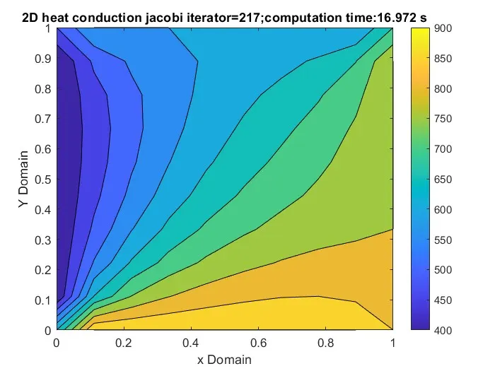
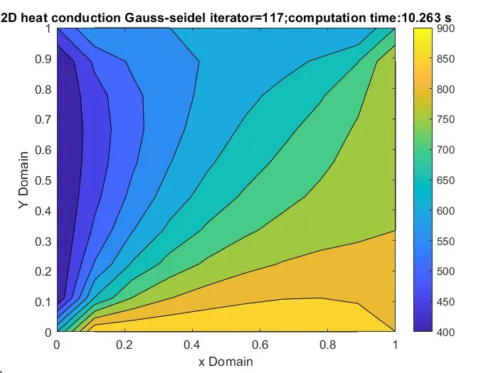
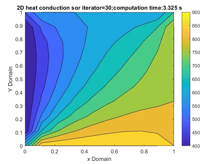
In the above three plot results you can see that the number of iterations and the computational time for jacobi method is high i.e 217 iterations and 24.193 seconds time and then it is for gauss seidel method with 117 iterations and 14.316 seconds time and then for SOR. on addition of over relaxiation factor to gauss seidel method i.e, SOR method we can see that the solution is calculated in just 30 iterations and 3.275 seconds time. The SOR method depends on relaxation factor and the solution is optimum with less number of iterations and computational time when the omega value is 1.5 and the above or below this the number iterations gets increased and when the value is above 1.99 the solution is getting blow up. So the maximum value of omega must be less than 2.
Descritized from of transient state conduction using explicit scheme:
This scheme is called the explicit scheme because it can solved diectly without resulting in a system of linear equations. Therefore, using ths scheme does not required iterative solvers
`(∂ T/ ∂ t) = ∝ (( ∂ ^2 T)/ (∂ x ^2 )+ (∂ ^2 T )/(∂ y ^2 ))`
`(T_(i-1,j)^(n+1)-T_(i,j)^n)/(Δt)=α((T_(i-1,j)-2T_i,_j+T_(i+1,j))/(Δx^2)+(T_(i,j-1)-2T_i,_j+T_(i,j+1))/(Δy^2))^n`
Let us consider `k1= α(Δt/Deltax^2)` and `k2= α(Δt/Deltay^2)`
By further simplification we can get
`T_(i,j)^(n+1)=T_i,_j(1-2k_1-2k_2)+k_1(T_(i-1,j)+T_(i+1,j))+k_2(T_(i,j-1)+T_(i,j+1))`
Here k1 and k2 resembles the CFL criteria which states that the CFL number should be <=0.5 to achiees stability.
k1=CFLx&k2=CFLy ==> CFLx+CFLy ≤0.5
From this condition we can get a range of values for dt(timestep)
MATLAB Code:
%explicit mtethod
clear all
close all
clc

l=1; % Length of the domain
nx=10;%define number of grid points in x_axis
ny=nx;%defines number of grid points in y_axis
x=linspace(0,1,nx);
y=linspace(0,1,ny);
dx=l/(nx-1);%grid spacing
dy=l/(ny-1);%grid spacing

% Define boundary conditions
top=600;
bottom=900;
left=400;
right=800;
% Initialize temperature matrix
T=ones(nx,ny);
T(1,2:nx-1)=top;
T(ny,2:nx-1)=bottom;
T(2:ny-1)=left;
T(2:ny-1,nx)=right;

T(1,1)=(top+left)/2;
T(1:1,nx)=(top+right)/2;
T(ny,1)=(bottom+left)/2;
T(ny,nx)=(right+bottom)/2;
told=T;% Initialize the previous temperature matrix

%simulation run time
t=0.4;
%time step
dt=1e-4;
%time step size
nt=t/dt;
omega=1.5;
k1=omega*(dt/dx^2);
k2=omega*(dt/dy^2);
k_coef=(1-(2*k1)-(2*k2));
CFL=omega*((dt/dx^2)+(dt/dy^2))
tic;
%time loop
for iter=1:nt;
    %space loop
    for i=2:nx-1;
        for j=2:ny-1;
        T(i,j)=k_coef*told(i,j)+k1*(told(i-1,j)+told(i+1,j))+k2*(told(i,j+1)+told(i,j-1));
        end
    end
    %update solution for next time step
    told=T;
    a=toc;
    contourf(x,fliplr(y),T)
    colorbar
    xlabel('x Domain')
    ylabel('y Domain')
    title_text=sprintf('2D heat conduction explict,time =%0.3f s',a);
    title(title_text);
    pause(0.03)
end
Output of solver:
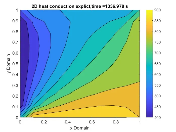
Here we get the solution when it satisfy the CFL number condition
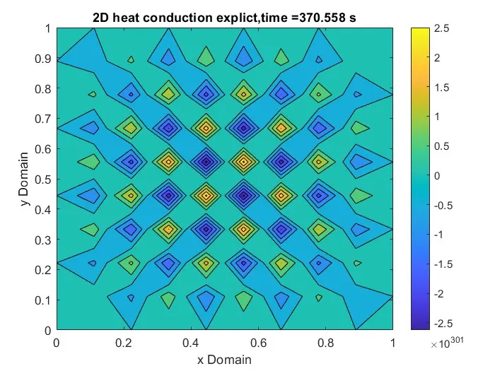
In this condition is satisfied the CFL number you see that the solution is blow up.
Descritized form of transient state conduction using implicit scheme
The implicit scheme however requires us to solve a system of coupled linear equations to get to the solution which makes it difficult to solve it using direct method. This is where the iterative solvers help us to solve such equations which less complexity and the results at desired level of accuracy, and in lesser time.
`(∂ T/ ∂ t) = ∝ (( ∂ ^2 T)/ (∂ x ^2 )+ (∂ ^2 T )/(∂ y ^2 ))`
`(T_(i-1,j)^(n+1)-T_i,_j^n)/(Δt)=α((T_(i-1,j)-2T_i,_j+T_(i+1,j))/(Δx^2)+(T_(i,j-1)-2T_i,_j+T_(i,j+1))/(Δy^2))^(n+1)`
let us consider `k1= α(Δt/Deltax^2)` and`k2= α(Δt/Deltay^2)`
By further simplification we can get
`T_(i,j)^(n+1) *(1+2k_1+2k_2)=T_(i,j)^n+k_1(T_(i-1,j)+T_(i+1,j))^(n+1)+k_2(T_(i,j-1)+T_(i,j+1))^(n+1)`
`T_(i,j)^(n+1) =(T_(i,j)^n+k_1(T_(i-1,j)+T_(i+1,j))^(n+1)+k_2(T_(i,j-1)+T_(i,j+1))^(n+1))/(1+2k_1+2k_2)`
Consider
term1=`1/(1+2k_1+2k_2)`
`term2=k_1*term1`
`term3=k_2*term1`
`T_(i,j)^(n+1)=term1*T_(i,j)^n+term2*(T_(i-1,j)+T_(i+1,j))^(n+1)+term3*(T_(i,j-1)+T_(i,j+1))^(n+1)`
MATLAB code:
%Using iterative technique solve the 2D heat conduction
%jacobi method
clear all
close all
clc

l=1;% Length of the domain
nx=10;%define number of grid points in x_axis
ny=nx;%defines number of grid points in y_axis
x=linspace(0,l,nx);
y=linspace(0,l,ny);

dx=l/(nx-1);%grid spacing
dy=l/(ny-1);%grid spacing
% Define boundary conditions
top=600;
bottom=900;
left=400;
right=800;
% Initialize temperature matrix
T=ones(nx,ny);
T(1,:)=top;
T(ny,:)=bottom;
T(:,nx)=right;
T(:,1)=left

T(1,1)=(left+top)/2;
T(1,nx)=(top+right)/2;
T(ny,1)=(left+bottom)/2;
T(ny,nx)=(right+bottom)/2;
Told=T;% Initialize the previous temperature matrix
Tprev=T
%simulation run time
t=0.4;
%time step
dt=1e-4;
%time step size
nt=t/dt;
error=9e-9;
tol=1e-4;
omega=1.5;
k1=omega*(dt/dx^2);
k2=omega*(dt/dy^2);
iterative_solvers=1;
tic
if iterative_solvers==1
    jacobi_iterator=1
    for m=1:nt;
        error=1;
        while (error>tol);
            term1=1/(1+(2*k1)+(2*k2));
            term2=k1*term1;
            term3=k2*term1;
            for i=2:nx-1;
                for j=2:ny-1;
                    H=(Told(i-1,j)+Told(i+1,j));
                    V=(Told(i,j+1)+Told(i,j-1));
                    T(i,j)=(Tprev(i,j)*term1+(H*term2)+(V*term3));
                end
            end
            % Calculate the maximum absolute difference between old and new temperature matrices
            error=max(max(abs(Told-T)));
            Told=T;
            jacobi_iterator=jacobi_iterator+1;
        end
        Tprev=T;
        time_required=toc
        % Display the current temperature distribution
        contourf(x,flip(y),T)
        colorbar
        xlabel('X Domain')
        ylabel('Y Domain')
        title_text=sprintf('2D heat conduction transient jacobi iterator=%d;computation time:%0.3f s',jacobi_iterator,time_required);
        title(title_text);
        pause(0.03)
    end
end
%Using iterative technique solve the 2D heat conduction
%Gauss-seidel method
clear all
close all
clc
l=1;% Length of the domain
nx=10;%define number of grid points in x_axis
ny=nx;%defines number of grid points in y_axis
x=linspace(0,l,nx);
y=linspace(0,l,ny);
dx=l/(nx-1);%grid spacing
dy=l/(ny-1);%grid spacing
% Define boundary conditions
top=600;
bottom=900;
left=400;
right=800;
% Initialize temperature matrix
T=ones(nx,ny);
T(1,:)=top;
T(ny,:)=bottom;
T(:,nx)=right;
T(:,1)=left
T(1,1)=(left+top)/2;
T(1,nx)=(top+right)/2;
T(ny,1)=(left+bottom)/2;
T(ny,nx)=(right+bottom)/2;
Told=T;% Initialize the previous temperature matrix
Tprev=T
%simulation run time
t=0.4;
%time step
dt=1e-4;
%time step size
nt=t/dt;
error=9e-9;
tol=1e-4;
omega=1.5;
k1=omega*(dt/dx^2);
k2=omega*(dt/dy^2);
iterative_solvers=1;
tic
if iterative_solvers==1
Gs_iterator=1
for m=1:nt;
error=1;
while (error>tol);
term1=1/(1+(2*k1)+(2*k2));
term2=k1*term1;
term3=k2*term1;
for i=2:nx-1;
for j=2:ny-1;
H=(Told(i-1,j)+Told(i+1,j));
V=(Told(i,j+1)+Told(i,j-1));
T(i,j)=(Tprev(i,j)*term1+(H*term2)+(V*term3));
end
end
% Calculate the maximum absolute difference between old and new temperature matrices
error=max(max(abs(Told-T)));
Told=T;
Gs_iterator=Gs_iterator+1;
end
Tprev=T;
time_required=toc
% Display the current temperature distribution
contourf(x,flip(y),T)
colorbar
xlabel('X Domain')
ylabel('Y Domain')
title_text=sprintf('2D heat conduction transient Gs iterator=%d;computation time:%0.3f s',Gs_iterator,time_required);
title(title_text);
pause(0.03)
end
endclear all
close all
clc
l=1;
nx=10;
ny=nx;
x=linspace(0,l,nx);
y=linspace(0,l,ny);
dx=l/(nx-1);
dy=l/(ny-1);
% Define boundary conditions
top=600;
bottom=900;
left=400;
right=800;
% Initialize temperature matrix
T=ones(nx,ny);
T(1,:)=top;
T(ny,:)=bottom;
T(:,nx)=right;
T(:,1)=left
T(1,1)=(left+top)/2;
T(1,nx)=(top+right)/2;
T(ny,1)=(left+bottom)/2;
T(ny,nx)=(right+bottom)/2;
Told=T;% Initialize the previous temperature matrix
Tprev=T
%simulation run time
t=0.4;
%time step
dt=1e-4;
%time step size
nt=t/dt;
error=9e-9;
tol=1e-4;
omega=1.0;
k1=omega*(dt/dx^2);
k2=omega*(dt/dy^2);
iterative_solvers=1;
tic
if iterative_solvers==1
sor_iterator=1
for m=1:nt;
error=1;
while (error>tol);
term1=1/(1+(2*k1)+(2*k2));
term2=k1*term1;
term3=k2*term1;
for i=2:nx-1;
for j=2:ny-1;
H=(T(i-1,j)+Told(i+1,j));
V=(Told(i,j+1)+T(i,j-1));
T1=omega*((Tprev(i,j)*term1+(H*term2)+(V*term3)));
T2=Told(i,j)*(1-omega);
T(i,j)=T1+T2;
end
end
% Calculate the maximum absolute difference between old and new temperature matrices
error=max(max(abs(Told-T)));
Told=T;
sor_iterator=sor_iterator+1;
end
Tprev=T;
time_required=toc
% Display the current temperature distribution
contourf(x,flip(y),T)
colorbar
xlabel('X Domain')
ylabel('Y Domain')
title_text=sprintf('2D heat conduction sor iterator=%d;computation time:%0.3f s',sor_iterator,time_required);
title(title_text);
pause(0.03)
end
endOutput of the solvers:
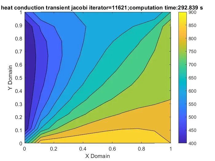
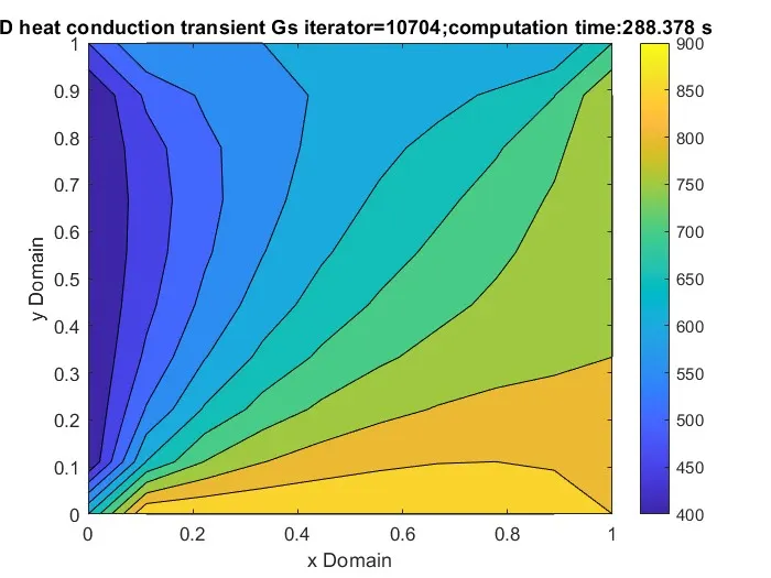
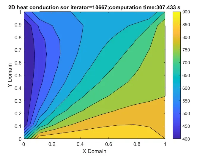
From the above plots you can conclude that explicit method takes more time to execute but when it comes to stability it mainly depends on CFL condition if this condition is not satisfied the simulation gets blow up. Where as in the implicit method jacobian method gives the solution in 11621 itrations where gauss method takes 10704 iterations but using SOR method you get the solution in 10667 iterations but the computational time high for the SOR ,Here SOR method if you can use omega value 1.01 you can see the iterations count increases when it crosses 1.99 then you see that the solution get blow up. So its value should be given less than 2. You can also observe that for any values of omega dx and dt solution will be stable, like explicit method it not dependent of CFL condition.