Week 5.1 - Mid term project - Solving the steady and unsteady 2D heat conduction problem
Aim:
The aim is to solve the 2D heat conduction dilemma under both steady and unsteady conditions, iterative methods such as Jacobi, Gauss-Seidel, and successive over-relaxation are employed.
Theory:
Conduction, a form of heat transfer, predominantly occurs within solids due to temperature disparities arising from the interplay between free electrons and lattice vibrations.
The below provided equation represents a generalized conduction model,
`(del^2 T)/ (delx^2) + (del^2 T)/ (dely^2) + (del^2 T)/ (delz^2) + (q/k) = 1/alpha ((delT)/(del tau))`
where,
T = Temperature
q = Heat generation
Alpha (a) = Thermal diffusivity
-
Thermal diffusivity is a thermophysical characteristic of a material, calculated as the ratio between its thermal conductivity and thermal capacity.
-
Given the problem's two-dimensional nature and the absence of heat generation, those terms are disregarded. As a result, the equation portrays the unsteady 2D heat conduction in a parabolic form.
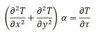
In a steady-state scenario, the time derivative is excluded. Therefore, the equation below delineates the depiction of two-dimensional steady-state heat conduction, characterized as elliptic.
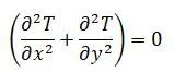
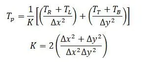
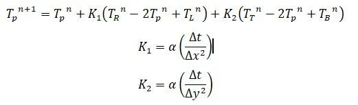
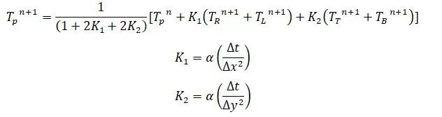
Difference equations are formulated to derive the numerical solutions for both the steady-state and unsteady-state two-dimensional conduction equations.
Steady State 2D heat conduction:
Transient 2D heat conduction (explicit):
Transient 2D heat conduction (implicit):
-
The approach employs iterative methods to solve the difference equation. Iterative methods are numerical strategies utilized to iteratively converge towards an accurate solution from an initial approximation.
-
Specifically, this process employs the Jacobi, Gauss-Seidel, and successive over-relaxation techniques.
Matlab code:
-
Two distinct MATLAB codes have been developed to handle steady and unsteady conditions.
-
It's important to note that the inputs remain consistent for both conditions.
-
During the programming process, the domain is conceptualized as a 1m by 1m surface, discretized into 10 nodes in both the horizontal and vertical directions.
-
The programming incorporates unchanging values, such as alpha and the time step 'data', while adhering to explicit conditions.
-
Additionally, the relaxation factor omega is exclusively assumed during the programming phase.
Inputs
| Top boundary temperature | 600 K |
| Bottom Boundary temperature | 900 K |
| Left Boundary temperature | 400 K |
| Right Boundary temperature | 800 K |
| error | 1e-4 |
- Initial inputs are assigned to variables, and a temperature array is established.
- Boundary conditions are incorporated into the temperature array, and average values are assigned to corner boundaries.
- Constants like alpha, omega, and tolerance are defined to facilitate the iteration process.
- User input is solicited to determine the preferred iterative method.
- An if-else loop is implemented to solve the equation using the user-selected iterative technique.
- A while loop is employed to execute the chosen iterative method until the desired level of accuracy is attained.
- Two nested for loops are utilized to compute temperature values for each node during every iterative step.
- Ultimately, the temperature distribution graph is generated using the 'contourf' command.
clear all
close all
clc

% Domain
number_node = 10;
% dicretization length
domain_length = 1;

%value of x and y at nodes in a discretization plane
x = linspace(0,domain_length,number_node);
y = linspace(0,domain_length,number_node);
dx = domain_length/(number_node-1);
dy = domain_length/(number_node-1);


% Let define a temperature value at all nodes with initial guess 300k
T = 300*ones(number_node,number_node);

% Initia boundary conditions at left and right
T(1:end,1) = 400;
T(1:end,end) = 800;

% Initia boundary conditions at bottom and top
T(end,1:end) = 900;
T(1,1:end) = 600;

%average values of T at corner boundaries
T(1,1) = 500;
T(end,1) = 650;
T(1,end) = 700;
T(end,end) = 850;

%copy of Temperature to compute to compute
T_old = T;

%constant
K = (2*(dx^2+dy^2))/(dx^2*dy^2);
omegha = 1.2;

% to enter while loop initialize error value randomly
error = 10;
tol = 1e-4;
no_iteration = 0;

method = input('Enter(1) for jacobi,(2) for gauss siediel,(3) for sos');
if method == 1
    while(error>tol)
        for i = 2:number_node-1
            for j = 2:number_node-1
            term1 = (T_old(i+1,j)+T_old(i-1,j))/dx^2;
            term2 = (T_old(i,j+1)+T_old(i,j-1))/dy^2;
            T(i,j) = (term1+term2)/K;
            end
        end
        error = max(max(abs(T_old-T)));

        % to upadte the previous velcity with new velocity
        %got from the iteration
        T_old = T;
        no_iteration = no_iteration+1;

    end
elseif method == 2
    while(error>tol)
        for i = 2:number_node-1
            for j = 2:number_node-1
            term1 = (T_old(i+1,j)+T(i-1,j))/dx^2;
            term2 = (T_old(i,j+1)+T(i,j-1))/dy^2;
            T(i,j) = (term1+term2)/K;
            end
        end
        error = max(max(abs(T_old-T)));

        % to upadte the previous velcity with new velocity
        %got from the iteration
        T_old = T;
        no_iteration = no_iteration+1;
    end

else
    while(error>tol)
        for i = 2:number_node-1
            for j = 2:number_node-1
            term1 = (T_old(i+1,j)+T(i-1,j))/dx^2;
            term2 = (T_old(i,j+1)+T(i,j-1))/dy^2;
            T(i,j) = ((1-omegha)*T_old(i,j))+(omegha*((term1+term2)/K));
            end
        end
        error = max(max(abs(T_old-T)));

        % to upadte the previous velcity with new velocity
        %got from the iteration
        T_old = T;
        no_iteration = no_iteration+1;

    end
end

% to visualize the result

[X,Y] = meshgrid(x,y);
contourf(X,Y,T)
colorbar
set(gca,'ydir','reverse')
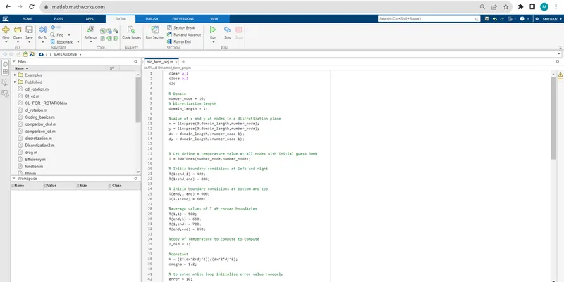
Matlab screenshot:
Unsteady-State 2D Heat conduction:
- Input values are assigned to variables, leading to the creation of a temperature array.
- The temperature array incorporates boundary conditions, with corner boundary values being averaged.
- Constants like alpha, omega, and tolerance are established to govern the iteration process.
- User interaction plays a pivotal role; the user must input one or two values.
- The initial input determines whether the problem should be solved using an explicit or implicit approach.
- When an implicit approach is chosen, a second input is required from the user to select the preferred iterative technique.
- An if-else loop is utilized to address the equation using the approach and iterative technique selected by the user.
- A for loop is employed to execute the iteration for a substantial number of cycles until reaching steady-state conditions.
- Meanwhile, a while loop runs the chosen iterative technique until the desired level of accuracy is achieved.
- Two nested for loops perform the computation of temperature values at each node for every iterative step.
- Ultimately, the outcome is visualized through a temperature distribution graph generated using the 'contourf' command.
clear all
close all
clc
% Domain and dicretization length
number_node = 10;
domain_length = 1;
%value of x and y at nodes in a discretization plane
x = linspace(0,domain_length,number_node);
y = linspace(0,domain_length,number_node);
dx = (domain_length/number_node-1);
dy = (domain_length/number_node-1);
dt = 1/10;
% Let define a temperature value at all nodes with initial guess 300k
T = 300*ones(number_node,number_node);
% Initia boundary conditions at left and right
T(1:end,1) = 400;
T(1:end,end) = 800;
% Initia boundary conditions at bottom and top
T(end,1:end) = 900;
T(1,1:end) = 600;
%average values of T at corner boundaries
T(1,1) = 500;
T(end,1) = 650;
T(1,end) = 700;
T(end,end) = 850;
%copy of Temperature to compute for previous space terms
T_old = T;
% copy of T for previous time_step
T_prev = T;
%constants
alpha = 1.5;
omegha = 1.15;
K1 = (alpha*dt)/(dx^2);
K2 = (alpha*dt)/(dy^2);
iteration = 0;
approach = input('Enter 1 for implicit or Enter 2 for explicit')
if approach == 1
method = input('Enter 1 for jacobi or 2 for gauss siedel or 3 for sos')
if method == 1
for nt = 1:1500
error = 10;
tol = 1e-4;
while(error>tol)
for i = 2:number_node-1
for j = 2:number_node-1
term1 = 1/(1+(2*K1)+(2*K2));
term2 = K1*(T_old(i+1,j)+T_old(i-1,j));
term3 = K2 *(T_old(i,j+1)+T_old(i,j-1));
T(i,j) = term1*(T_prev(i,j)+term2+term3);
end
end
iteration = iteration+1;
error = max(max((abs(T_old-T))));
T_old = T;
end
T_prev = T;
end
elseif method ==2
for nt = 1:1500
error = 10;
tol = 1e-4;
while(error>tol)
for i = 2:number_node-1
for j = 2:number_node-1
term1 = 1/(1+(2*K1)+(2*K2));
term2 = K1*(T_old(i+1,j)+T(i-1,j));
term3 = K2 *(T_old(i,j+1)+T(i,j-1));
T(i,j) = term1*(T_prev(i,j)+term2+term3);
end
end
iteration = iteration+1;
error = max(max(abs(T_old-T)));
T_old = T;
end
T_prev = T;
end
else
for nt = 1:1500
error = 10;
tol = 1e-4;
while(error>tol)
for i = 2:number_node-1
for j = 2:number_node-1
term1 = 1/(1+(2*K1)+(2*K2));
term2 = K1*(T_old(i+1,j)+T(i-1,j));
term3 = K2 *(T_old(i,j+1)+T(i,j-1));
term4 = term1*(T_prev(i,j)+term2+term3);
T(i,j)=(1-omegha)*T_old(i,j)+(omegha*term4);
end
end
iteration = iteration+1;
error = max(max(abs(T_old-T)));
T_old = T;
end
T_prev = T;
end
end
else
for nt = 1:1500
for i = 2:number_node-1
for j = 2:number_node-1
term1 = K1*(T_prev(i+1,j)-2*T_prev(i,j)+T_prev(i-1,j));
term2 = K2*(T_prev(i,j+1)-2*T_prev(i,j)+T_prev(i,j-1));
T(i,j) = T_prev(i,j)+term1+term2;
end
end
% to upadte the previous timestep value with new timestep value
%got from the iteration
T_prev = T;
iteration = iteration+1;
end
end
% to visualize the result
[X,Y] = meshgrid(x,y);
figure(1)
contourf(X,Y,T)
colorbar
set(gca,'ydir','reverse')
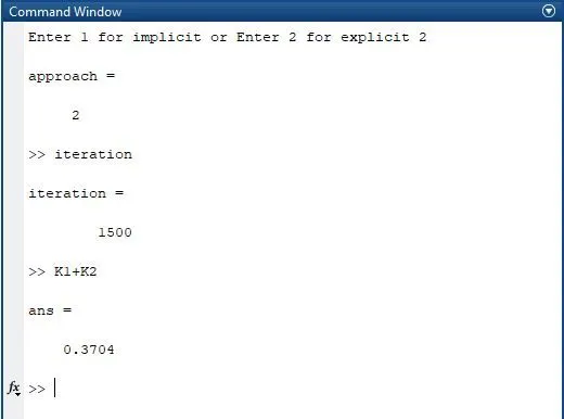
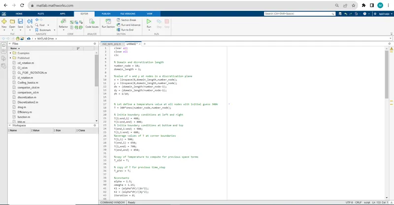
Matlab screenshot:
RESULT:
-
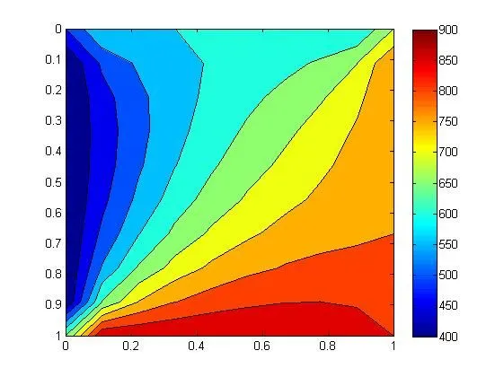
The program executes without any issues, yielding identical temperature distribution plots for both steady and unsteady conditions.
-
This equivalence arises from the fact that even in transient analysis, the solution gradually converges towards the steady-state outcome.
-
Notably, the upper, lower, left, and right sides of the graphs correspondingly symbolize their respective boundary conditions
-
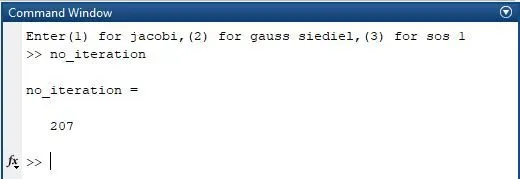
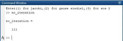
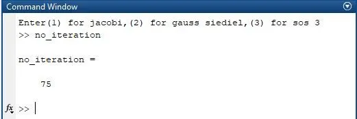
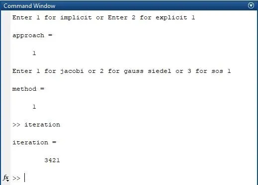
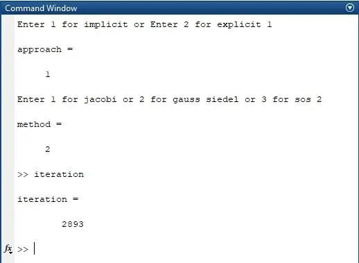
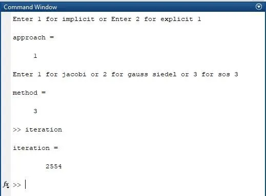
A comparison is drawn regarding the quantity of iterations necessary for the three iterative techniques to attain convergence to the solution.
-
In both the steady and transient analyses, the Successive Over-Relaxation method outperforms, requiring a lower number of iterations.
-
Specifically, the Successive Over-Relaxation technique demands fewer iterations to reach convergence.
Steady-State analysis:
- Jacobi
- Gauss-Siedel
- Successive over relaxation
Transient analysis - Out of a number of iterations -> 1500 iterations is due to time step
- Jacobi
- Gauss-Siedel
- Successive over-relaxation
Explicit
1500 iterations are due to time step. According to CFL stability criteria,
K1+K2<0.5.