Week 5.1 - Mid term project - Solving the steady and unsteady 2D heat conduction problem

                                              STEADY AND UNSTEADY 2D HEAT CONDUCTION PROBLEM

AIM:

To Solve the 2D heat conduction equation for steady state analysis and transient state analysis by using the point iterative techniques .

OBJECTIVE;

To write code for both implicit and explicit schemes for the transient analysis only.

To compare the convergence rate [Number of iterations] of the steady state and transient [explicit and implicit] simulations and justify the numerics.

[Implement the following methods for solving implicit equations ,Jacobi,Gauss-seidel,Successive over-relaxation].

Input Parameters;

The Boundary conditions for the problem are as follows;

Top Boundary = 600 K

Bottom Boundary = 900 K

Left Boundary = 400 K

Right Boundary = 800 K

Absolute error criteria is 1e-4

ASSUMPTIONS:

Consider a Square domain of 1 m length

EQUATIONS;

2D heat equation for steady state condition

`(del^2T)/(del^2x) + (del^2T)/(del^2y) = 0`

2D heat conduction equation for transient condition

`(delT)/(delt) + alpha((del^2T)/(del^2x) + (del^2T)/(del^2y)) = 0`

THEORY:

1. Steady state analysis & Transient State Analysis

The heat conduction eqautions has been solved using explicit & implicit method. In steady state condition, the equations has been solved using only implicit method while in transient condition, equations will be solved using both methods.

In explicit method, the current node values has been calculated based on the values calculated in previous time step. The Courant Numbers or the CFL value is very important in explicit method to maintain the stability while implementing it. The values should be below 0.5 to maintain the stability of the process. The CFL values has been determined which will be presented in the respective section. 

The implicit method try to seek the value of the next node and the values of each variable on that node has not been determined while implementing implicit method on the current node. To determine the values on the next node in mesh, iterative method has been used. Three methods has been implemented to compare their peroformance in terms of numner of iterations & time taken by each method to evaluate their effectiveness. 

Following three methods, with their short introduction about working, has been used:

a) Jacobi Iterative method

This method is used to solve linear equation by point-wise iteration method. Jacobi method uses the values determined in the previus time step to solve the equations in current  iteration.

b) Gauss Seidel (GS) Iterative method

Gauss seidel method is also similar to jacobi iterative method in terms of performing iteration by point-wise method. But in contrast to jacobi, this method uses the latest updated values to solve the linear equation.

c) Successive Over Relaxation (SOR) iterative method

SOR is not an independent method like previous two, but this method has been variant of GS method to improve the performance of the iterative method. This method can be implemented to solve the linear equation with either of the two previously defined method with addition to relaxation factor which helps in improving the performance of the method.

1.1 Steady State Condition

From the given boundary conditions, temperature will be calculated at the centre of the domain using following equation:

`T_p = 1/k (((T_L + T_R)/(del^2x)) + ((T_T + T_B)/(del^2y)))`

 MATLAB Syntax for Jacobi Method:

%Jacobi Iterative Method for Implicit function

function [out] = jacobi_method(T,k,tol,Told,error,nx,ny,dx,dy,xx,yy)

%solving 2d heat conduction equation for steady state condition

tic;   % start time

jacobi_method=1;
while (error > tol ) % program will stop if this criteria is achieved
    for i = 2:nx-1
        for j =2:ny-1

            %splitting the equation in two terms
            t1 = ((Told(i-1,j) + Told(i+1,j))/(dx^2))/k;
            t2 = ((Told(i,j-1) + Told(i,j+1))/(dy^2))/k;
            T(i,j) = t1+t2;
        end
    end
    error = max(max(abs(Told-T)));
    Told = T;

    %Defining the incrementation for iteration
    jacobi_method = jacobi_method+1;
    %to stop time
    sol_time_jacobi = toc;

    %plotting temperature distribution
    figure(1)
    %plotting contour graph
    [a,b] = contourf(xx,yy,T);
    %labelling each curve in contour graph for a & b
    clabel(a,b)
    %chart color pattern
    colormap(autumn)
    %Enable color bar
    colorbar

    %setting y axis in reverse order
    set(gca,'ydir','reverse')
    %Insert title
    title(sprintf('jacobi method = %d\n Iteration time = %f sec',jacobi_method,sol_time_jacobi))
    %Display x & y labels
    xlabel('X Axis')
    ylabel('Y Axis')

end

out = sol_time_jacobi

end

MATLAB Syntax for Gauss seidel Method:

%Gauss seidel Iterative Method for Implicit function

function [out] = gauss_method(T,k,tol,Told,error,nx,ny,dx,dy,xx,yy)

%solving 2d heat conduction equation for steady state condition
%Gauss Seidel Implicit Method

tic;   % start time

gauss_method=1;
while (error > tol ) % program will stop if this criteria is achieved
    for i = 2:nx-1
        for j =2:ny-1

            %splitting the equation in two terms
            t1 = ((Told(i-1,j) + Told(i+1,j))/(k*dx^2));
            t2 = ((Told(i,j-1) + Told(i,j+1))/(k*dy^2));
            T(i,j) = t1+t2;
        end
    end
    error = max(max(abs(Told-T)));
    Told = T;

    %Defining the incrementation for iteration
    gauss_method = gauss_method+1;
    %to stop time
    sol_time_gauss = toc;

    %plotting temperature distribution
    figure(2)
    %plotting contour graph
    [a,b] = contourf(xx,yy,T);
    %labelling each curve in contour graph for a & b
    clabel(a,b)
    %chart color pattern
    colormap(summer)
    %Enable color bar
    colorbar

    %setting y axis in reverse order
    set(gca,'ydir','reverse')
    %Insert title
    title(sprintf('gauss seidel method = %d\n Iteration time = %f sec',gauss_method,sol_time_gauss))
    %Display x & y labels
    xlabel('X Axis')
    ylabel('Y Axis')

end

out = sol_time_gauss

end

MATLAB Syntax for SOR Method:

%Successive Over Relaxation method using Gauss-seidel Iterative Method for 
% Implicit function

function [out] = sor_method(T,k,tol,Told,error,nx,ny,dx,dy,xx,yy)

%solving 2d heat conduction equation for steady state condition
%Successive over relaxation Implicit Method

omega = 1.2;

tic;   % start time

sor_method=1;
while (error > tol ) % program will stop if this criteria is achieved
    for i = 2:nx-1
        for j =2:ny-1

            %splitting the equation in two terms
            t1 = ((T(i-1,j) + T(i+1,j))/(k*dx^2));
            t2 = ((T(i,j-1) + T(i,j+1))/(k*dy^2));
            T_GS = t1 + t2;
            T(i,j) = (1-omega)*(Told(i,j)) + omega*(T_GS);
        end
    end
    error = max(max(abs(Told-T)));
    Told = T;

    %Defining the incrementation for iteration
    sor_method = sor_method+1;
    %to stop time
    sol_time_sor = toc;

    %plotting temperature distribution
    figure(3)
    %plotting contour graph
    [a,b] = contourf(xx,yy,T);
    %labelling each curve in contour graph for a & b
    clabel(a,b)
    %chart color pattern
    colormap(winter)
    %Enable color bar
    colorbar

    %setting y axis in reverse order
    set(gca,'ydir','reverse')
    %Insert title
    title(sprintf('SOR method = %d\n Iteration time = %f sec',sor_method,sol_time_sor))
    %Display x & y labels
    xlabel('X Axis')
    ylabel('Y Axis')

end

out = sol_time_sor

end

MAIN SYNTAX for Implicit steady state condition

%solving 2D heat conduction equation for Implicit scheme
%for steady state condition

clear all
close all
clc

%Input Parameters
nx = 10;
ny = nx;
l = 1; % ;length of square domain

% Creating mesh

x = linspace(0,l,nx);
y = linspace(0,l,ny);
dx = x(2) -x(1); % time step size in x
dy = dx; % time atep size in y
[xx,yy] = meshgrid(x,y);

%Initial value of the error
error = 9e9;
tol = 1e-4; %tolerance value

%calculating constant "k"
k = 2*((1/dx^2)+(1/dy^2));

%Boundary conditions
T = ones(nx,ny);
%inserting temperature values at different side of the domain
T(:,1) = 400; %Left boundary
T(1,:) = 600; %Top boundary
T(:,end) = 800; % right boundary
T(end,:) = 900; % bottom boundary

%calculating the temperaturee at nodes
T(1,1) = (600+400)/2;
T(1,end) = (800+600)/2;
T(end,1) = (400+900)/2;
T(end,end) = (800+900)/2;

%Told = temperature during previous iteration
Told = T;

%Defining loop to execute solvers
for iter_solver = 1:3
    if iter_solver == 1  % for jacobi iterative method

        %calling Jacobi Iterative method
        jacobi_sol = jacobi_method(T,k,tol,Told,error,nx,ny,dx,dy,xx,yy);

    elseif iter_solver == 2 % For Gauss Seidel Iterative Method

        %calling Gauss seidel Iterative method
        gauss_sol = gauss_method(T,k,tol,Told,error,nx,ny,dx,dy,xx,yy);

    elseif iter_solver == 3 % For Successive Over relaxation Iterative Method

        %calling successive over relaxation Iterative method
        sor_sol = sor_method(T,k,tol,Told,error,nx,ny,dx,dy,xx,yy);
    end
end

RESULTS:

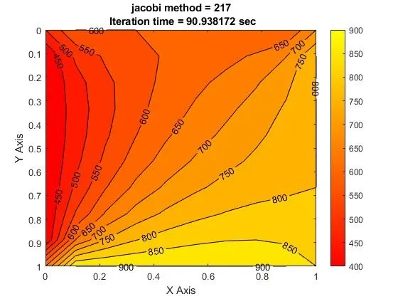
Jacobi Method

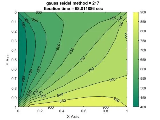
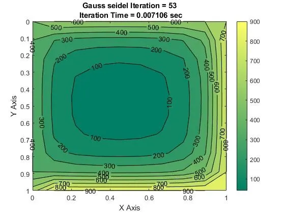
Gauss Seidel Method

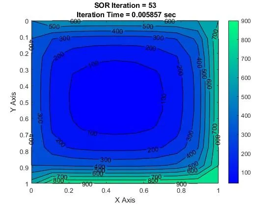
SOR Method

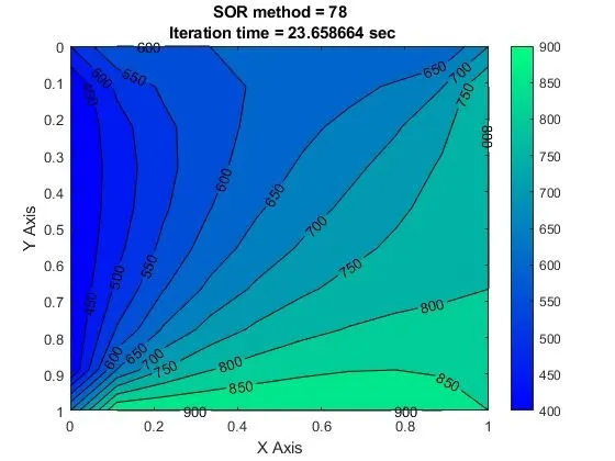
From the above plot, we can observe that the iterations are same for both gauss and jacobi method and gauss seidel method took less computational time than the jacobi method. Notably the no of iterations and the computational time is much less fo sor method.  

MATLAB Syntax for Jacobi Method:

%Wrirting Function for Jacobi Ierative method

function [out] = jacobi_tmethod(error, tol,k1, k2,nx, ny,T,Told,Tprev, xx,yy, nt)
%solving Jacobi method for Transient condition

tic; %start time

jacobi_iter = 1;

for k = 1:nt
    while (error > tol)
        for i = 2: nx-1
             for j = 2:ny-1
            t1 = 1/(1 + 2*k1 + 2*k2);
            t2 = k1*t1;
            t3 = k2*t1;
            H = Told(i-1,j) + Told(i+1,j);
            V = (Told(i,j-1) + Told(i,j+1));
            T(i,j) = Tprev(i,j)*t1 + H*t2 + V*t3;
        end
    end
    error = max(max(abs(Told-T)));
    Told = T;
    jacobi_iter = jacobi_iter+1;
    sol_time_jacobi = toc; %stop time and save
end
Tprev = T;
out =sol_time_jacobi;
end

figure(1)
[a,b] = contourf(xx,yy,T);
clabel(a,b)
colormap(autumn)
colorbar

set(gca,'ydir','reverse')
title(sprintf('Jacobi Iteration = %d\n Iteration Time = %f sec',jacobi_iter,sol_time_jacobi))
xlabel('X Axis')
ylabel('Y Axis')

end

MATLAB Syntax for Gauss seidel Method:

%Wrirting Function for Gauss seidel Ierative method

function [out] = gauss_tmethod(error, tol,k1, k2,nx, ny,T,Told,Tprev, xx,yy, nt)
%solving Gauss seidel method for Transient condition

tic; %start time

gauss_iter = 1;

for k = 1:nt
    while (error > tol)
        for i = 2: nx-1
             for j = 2:ny-1
            t1 = 1/(1 + 2*k1 + 2*k2);
            t2 = k1*t1;
            t3 = k2*t1;
            H = Told(i-1,j) + Told(i+1,j);
            V = (Told(i,j-1) + Told(i,j+1));
            T(i,j) = Tprev(i,j)*t1 + H*t2 + V*t3;
        end
    end
    error = max(max(abs(Told-T)));
    Told = T;
    gauss_iter = gauss_iter+1;
    sol_time_gauss = toc; %stop time and save
end
Tprev = T;
out =sol_time_gauss;
end

figure(2)
[a,b] = contourf(xx,yy,T);
clabel(a,b)
colormap(summer)
colorbar

set(gca,'ydir','reverse')
title(sprintf('Gauss seidel Iteration = %d\n Iteration Time = %f sec',gauss_iter,sol_time_gauss))
xlabel('X Axis')
ylabel('Y Axis')

end

MATLAB Syntax for SOR Method:

%Wrirting Function for SOR Ierative method

function [out] = sor_tmethod(error, tol,k1, k2,nx, ny,T,Told,Tprev, xx,yy, nt)
%solving SOR method for Transient condition

tic; %start time

sor_iter = 1;

for k = 1:nt
    while (error > tol)
        for i = 2: nx-1
             for j = 2:ny-1
            t1 = 1/(1 + 2*k1 + 2*k2);
            t2 = k1*t1;
            t3 = k2*t1;
            H = Told(i-1,j) + Told(i+1,j);
            V = (Told(i,j-1) + Told(i,j+1));
            T(i,j) = Tprev(i,j)*t1 + H*t2 + V*t3;
        end
    end
    error = max(max(abs(Told-T)));
    Told = T;
    sor_iter = sor_iter+1;
    sol_time_sor = toc; %stop time and save
end
Tprev = T;
out =sol_time_sor;
end

figure(3)
[a,b] = contourf(xx,yy,T);
clabel(a,b)
colormap(winter)
colorbar

set(gca,'ydir','reverse')
title(sprintf('SOR Iteration = %d\n Iteration Time = %f sec',sor_iter,sol_time_sor))
xlabel('X Axis')
ylabel('Y Axis')

end

MAIN SYNTAX FOR TRANSIENT IMPLICIT SCHEME:

%solving 2D heat conduction equation Implicit scheme
% for Transient condition

clear all
close all
clc

%Inputs & Grid points
nx=10;
ny=nx;
l=1; %length of the square domain
nt=1400; %number of timesteps


%creating mesh
x=linspace(0,1,nx); %no of nodes in x direction
y=linspace(0,1,ny); %no of nodes in y direction
dx = x(2) -x(1); %x timestep
dy = dx; %y timestep
[xx,yy] = meshgrid(x,y); %mesh grid

%Initial value of the error
error = 9e9;
tol = 1e-4; %tolerance value
dt = 0.01; %timestep
alpha = 1.4; %diffusivity


%calculating courant number (CFL values)
k1 = alpha*(dt/(dx^2));
k2 = alpha*(dt/(dy^2));

%boundary conditions
T = ones(nx,ny);
% temperature value at different domain
T(:,1) = 400;     %left boundary
T(1,:) = 600;     %Top boundary
T(:,end) = 800;   %Right boundary
T(end,:) = 900;   %Bottom boundary

%calculating 4 corner nodes temperature values
T(1,1) = (600+400)/2;
T(1,end) = (800+600)/2;
T(end,1) = (400+900)/2;
T(end,end) = (800+900)/2;

Tprev = T; %value of previous time step
Told = T;  %value of previous iteration

for iter_tsolver = 1:3
    if iter_tsolver == 1  % for Jacobi Iterative method
        
        %calling jacobi function
        jacobi_tsol = jacobi_tmethod(error, tol,k1, k2,nx, ny,T,Told,Tprev, xx,yy, nt)

    elseif iter_tsolver ==2 %for gauss seidel method
        
        %calling gauss transient function
        gauss_tsol = gauss_tmethod(error, tol,k1, k2,nx, ny,T,Told,Tprev, xx,yy, nt)

    elseif iter_tsolver ==3 %for sor method

        %calling sor transient function
        sor_tsol = sor_tmethod(error, tol,k1, k2,nx, ny,T,Told,Tprev, xx,yy, nt)
    end
end

RESULTS:

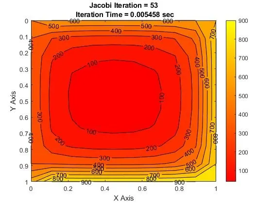
Jacobi method

Gauss Seidel Method

SOR Method

It is inferred that the jacobi method for transient implicit scheme is efficient and takes less time to solve than the other two methods. Out of this, gauss seeidel method takes more iteration time.

MATLAB syntax for Explicit scheme Transient condtion;

% 2D heat conduction equations explicit Scheme
% for Transient condition

clear all
close all
clc

% Square domain points
nx = 10;
ny = nx;
l = 1; % length of square domain
nt = 1400;


% Creating mesh
x = linspace(0,l,nx);
y = linspace(0,l,ny);
dx = x(2) - x(1); % step size in x
dy = dx; % step size in y
[xx,yy] = meshgrid(x,y); % mesh grid

% Initial value of the error
error = 9e9; 
tol = 1e-4; % tolerance value
dt = 0.001;
alpha = 1.4; % diffusivity


% Calculating Courant Numbers (CFL numbers)
k1 = alpha*(dt/(dx^2))
k2 = alpha*(dt/(dy^2))

% Boundary Conditions
T = ones(nx,ny);
% inserting temperature values at different side of the domain
T(:,1) = 400; % Left boundary 
T(1,:) = 600; % Top boundary
T(:,end) = 800; % Right boundary
T(end,:) = 900; % Bottom boundary


T(1,1) = (600 + 400)/2;
T(1,end) = (800 + 600)/2;
T(end,1) = (400 + 900)/2;
T(end,end) = (800 + 900)/2;

% Tprev = T; % value of previous time step
Told = T; % value of previous iteration

tic; % start timer
explicit_method = 1;
while (error > tol)
    for k = 1:nt
        for i = 2: nx-1
            for j = 2:ny-1
%                 t1 = 1/(1 + 2*k1 + 2*k2);
%                 t2 = k1*t1;t3 = k2*t1;
%                 H = Told(i-1,j) + Told(i+1,j);V = (Told(i,j-1) + Told(i,j+1));
%                 T(i,j) = Tprev(i,j)*t1 + H*t2 + V*t3;
                  T(i,j) = Told(i,j) + k1*(Told(i-1,j) - 2*Told(i,j) + Told(i+1,j) + ...
                      k2*(Told(i,j-1) - 2*Told(i,j) + Told(i,j+1)));
            end
        end
%         error = max(max(abs(Told - T)));
        error = max(abs(Told - T));
        Told = T;
        explicit_method = explicit_method + 1;
%         sol_time_explicit = toc; % stop timer & saving time into variable
    end
end

sol_time_explicit = toc; % stop timer

figure(1)
[a,b] = contourf(xx,yy,T);
clabel(a,b)
colormap(autumn)
colorbar

set(gca,'ydir','reverse')
title(sprintf('Explicit Method Iteration = %d\n Iteration Time = %f sec', ...
    explicit_method,sol_time_explicit ))
xlabel('X Axis')
ylabel('Y Axis')

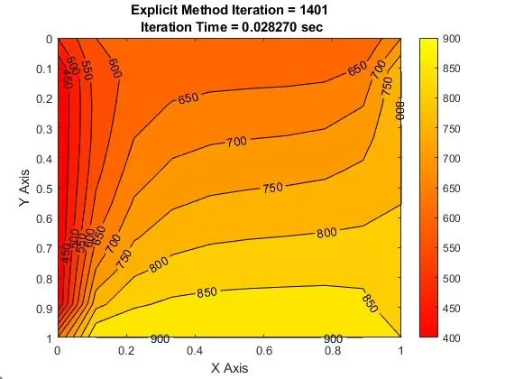
Courant Number k1 = 0.1134

Courant Number k2 = 0.1134

CONCLUSION:

By observing the data from the above plot, we can conclude by saying tht hte time taken and the no of iterations to solve the equations is more than the implicit scheme of both steady and transient conditions. Hence based on the problem we can choose the scheme and flow conditions to analyse the problem.