Week 5.1 - Mid term project - Solving the steady and unsteady 2D heat conduction problem
AIM
To perform Steady state analysis & Transient State Analysis to solve the 2D heat conduction equation by using the point and line iterative techniques such as Jacobi, Gauss-Seidel and Successive over-relaxation and compare the convergence rate of the steady state and transient [explicit and implicit] simulations.
INTRODUCTION
The governing equations in fluid mechanics and heat transfer can be reduced to elliptic, hyperbolic and parabolic forms for particular applications. Such examples are the steady-state heat conduction equation without internal heat generation or which is also called as the Laplace equation which is of elliptic form, steady-state heat conduction equation with internal heat generation or which is also called as the Poisson equation which is of hyperbolic form, etc. These model equations are used to investigate a variety of solution procedures. In this challenge we consider both steady and transient analysis of 2D heat conduction equation i.e., `(partial^2 T)/ (partial x^2) + (partial^2 T)/ (partial y^2)= 0` for steady state analysis `(partial^2 T)/ (partial x^2) + (partial^2 T)/ (partial y^2)= a * (partialT)/(partialt)` for transient analysis ........ 1
Solution Algorithms - In general, there are two methods of solution for the system of simultaneous linear algebraic equations. These schemes are classified as direct or iterative methods. Some familiar direct methods are Cramer's rule and Gaussian elimination. The major disadvantage of these methods is the enormous amount of arithmetic operations required to produce a solution.
Iterative procedures for solving a system of linear algebraic equations are simple and easy to program. The idea behind these methods is to obtain the solution by iteration. Usually an initial solution is guessed and new values are computed; based on the newly computed values, a newer solution is sought, and the procedure is repeated until a specified convergence criterion has been reached. egories. If a formulation results in only one unknown, then it is called a point iterative method. This formulation is similar to the explicit methods of parabolic equations. On the other hand, if the formulation involves more than one unknown it is classified as a line iterative method, which is similar to an implicit formulation of a parabolic equation.
- The Jacobi Iteration Method - In this method, the dependent variable at each grid point is solved, using initial guessed values of the neighboring points or previously computed values. The computation is carried out until a specified
convergence criterion is met. - The Point Gauss-Seidel Iteration Method - In this method, the current values of the dependent variable are used to compute the neighboring points as soon as they are available. This will certainly increase the convergence rate dramatically over the Jacobi method. The method is convergent if the largest elements are located in the main diagonal of the coefficient matrix.
- The Line Gauss-Seidel Iteration Method - This method converges faster than the point Gauss-Seidel method (by about a factor of 1/2), but it requires more computation time per iteration, since a system of simultaneous equations is being solved.
- Point Successive Over-Relaxation Method (PSOR) - If, during the solution process of computing the temperature distribution, a trend in the computed values of the dependent variable is noticed, then the direction of change can be used to extrapolate for the next iteration and, thereby, accelerate the solution procedure. This procedure is known as successive over-relaxation (SOR). As the solution proceeds, T(i,j) at n'th time step must approach T(i,j) at (n+1)'th time step. To accelerate the solution, we make use of the relaxation factor (w). For the solution to converge, it is necessary that 0 < w < 2. If 0 < w < 1, it is called under-relaxation. In this problem I have used a relaxation parameter of 1.205
- Line Successive Over-Relaxation Method (LSOR) - The line Gauss-Seidel iteration method can be accelerated by introducing a relaxation factor (w) similar to the one introduced into the point Gauss-Seidel method to provide the point SOR method. This method is called Line Successive Over-Relaxation Method.
Solution procedure for the implementation of these iterative methods to 2D heat conduction equation -
- We first discretize the fluid domain in both x and y directions assuming the grid size to be uniform in both the directions. In this problem I have chosen 10 segments in both x and y directions. We need to consider the stability criteria while using explicit scheme as very fine grid might exceed the Courant number and CFL criteria.
- We then discretize the equation 1 using central difference scheme for the spatial derivative and forward difference scheme for the time derivative to get a solution from the neighbouring points.
- Define the boundary and initial conditions at t = 0. Here we have used Dirchlet BC's.
- We need to define time step size considering the CFL criteria which states that the sum of the ratio of the product of distance travelled by the fluid in a single time step to the grid size in both x and y directions should be less than or equal to 0.5
- We also need to define various constants such as thermal diffusivity, relaxation factors, etc.
- Define a tolerance limit of 1e-4 (as per the problem statement) which is sufficient for convergence. We define an error term which is the difference between the initial guessed value and the current numerical value. If the error drops below the defined convergence criteria, we consider the solution to have attained steady state.
- We then compare the number of iterations required by the iterative methods to converge with the help of contour plots.
CODE AND OUTPUT
%%%% Steady state analysis of 2D heat conduction equation %%%%

close all
clear
clc

%% Discretizing the fluid domain

nx = 10;
ny = 10;
x = linspace(0,1,nx); % discretizing the domain in x-direction into 10 equal parts
y = linspace(0,1,ny); % discretizing the domain in y-direction into 10 equal parts
dx = x(2) - x(1); % grid size in x-direction
dy = y(2) - y(1); % grid size in y-direction

%% Implementing boundary and initial conditions

T = 300*ones(nx,ny); % initial temperature at all the 10x10 grid points
T(1,1) = 650; % temperature at grid point x = 1 and y = 1
T(1,ny) = 850; % temperature at grid point x = 1 and y = 10
T(nx,1) = 500; % temperature at grid point x = 10 and y = 1
T(nx,ny) = 700; % temperature at grid point x = 10 and y = 10
T(1,2:ny-1) = 900; % temperature at grid point x = 1 and y = 2 to y = 9
T(2:nx-1,1) = 400; % temperature at grid point x = 2 to x = 9 and y = 1
T(nx,2:ny-1) = 600; % temperature at grid point x = 10 and y = 2 to y = 9
T(2:nx-1,ny) = 800; % temperature at grid point x = 2 to x = 9 and y = 10
T_old = T;


k = 2*(((dx^2) + (dy^2))/((dx^2) * (dy^2)));
w = 1.2; % relaxation factor
tol = 1e-4; % absolute error criteria
error = 100; % initial error

method = input('Iterative method = '); %iterative method selection


%% JACOBI ITERATIVE METHOD

if (method==1)

jac_iter = 1; % initializing the iteration for Jacobi method

while (error > tol) % convergence limit

    for i = 2:nx-1

        for j = 2:ny-1

            % discretized equation to compute the temperature at a given
            % grid point using the initial values
            T(i,j) = (((T_old(i-1,j) + T_old(i+1,j))/dx^2) + ((T_old(i,j-1) + T_old(i,j+1))/dy^2)) * (1/k);


        end
    end

    error = max(max(abs(T_old - T))); % error computation
    T_old = T; % updating the old temperature with the current computed temperature
    jac_iter = jac_iter + 1; % incrementing the Jacobi iteration


end

figure(1)
colormap("jet")
contourf(x,y,T) % Temperature contour plot

end

%% GAUSS SEIDEL ITERATIVE METHOD

if (method==2)

GS_iter = 1; % initializing the iteration for GS method

while (error > tol) % convergence limit

    for i = 2:nx-1

        for j = 2:ny-1

            % discretized equation to compute the temperature at a given
            % grid point using the initial values and the computed vlues
            T(i,j) = (((T(i-1,j) + T_old(i+1,j))/dx^2) + ((T(i,j-1) + T_old(i,j+1))/dy^2)) * (1/k);


        end
    end

    error = max(max(abs(T_old - T))); % error computation
    T_old = T; % updating the old temperature with the current computed temperature
    GS_iter = GS_iter + 1; % incrementing the GS iteration


end


figure(2)
colormap("jet")
contourf(x,y,T) % Temperature contour plot
end

%% SUCCESSIVE OVER RELAXATION ITERATIVE METHOD

if (method==3)


SOR_iter = 1; % initializing the iteration for SOR method
while (error > tol) % convergence limit

    for i = 2:nx-1

        for j = 2:ny-1

           TGS = (((T(i-1,j) + T_old(i+1,j))/dx^2) + ((T(i,j-1) + T_old(i,j+1))/dy^2)) * (1/k);
            % discretized equation to compute the temperature at a given
            % grid point using the initial values and the computed vlues using relaxation factor to
            % accelerate the solution
           T(i,j) = ((1 - w) * T_old(i,j)) + (w*TGS);

        end
    end
    error = max(max(abs(T_old - T))); % error computation
    T_old = T; % updating the old temperature with the current computed temperature
    SOR_iter = SOR_iter + 1; % incrementing the SOR iteration
end
figure(3)
colormap("jet")
contourf(x,y,T) % Temperature contour plot
end

%%%% Transient state analysis of 2D heat conduction equation using explicit scheme%%%%

close all
clear
clc

nx = 10;
ny = 10;
x = linspace(0,1,nx);
y = linspace(0,1,ny);
dx = x(2) - x(1);
dy = y(2) - y(1);

T = 300*ones(nx,ny);
T(1,1) = 650;
T(1,ny) = 850;
T(nx,1) = 500;
T(nx,ny) = 700;
T(1,2:ny-1) = 900;
T(2:nx-1,1) = 400;
T(nx,2:ny-1) = 600;
T(2:nx-1,ny) = 800;
T_old = T;

a = 1.4; % thermal diffusivity
dt = 0.002; % time step
K1 = (a*dt)/dx^2; % CFL criteria in the x-diretion
K2 = (a*dt)/dy^2; % CFL criteria in the y-diretion
CFL = K1 + K2; % Validating the CFL criteria to be less than 0.5
w = 1.2; % relaxation factor

method = input('Iterative method = '); %iterative method selection

%% JACOBI METHOD

if (method == 1)
for k = 1:200 % for loop to compute temperature for 1000 time steps for the solution to reach steady state
    for i = 2:nx-1

        for j = 2:ny-1

            % discretized equation to compute the temperature at a given
            % grid point using the initial values at a given time step
            T(i,j) = (T_old(i,j)*(1-2*K1-2*K2)) + K1*(T_old(i+1,j)+T_old(i-1,j)) + K2*(T_old(i,j+1)+T_old(i,j-1));

        end

    end

    T_old = T; % updating the old values with the computed values

end
figure(1)
colormap("jet")
contourf(x,y,T)
end

%% GS METHOD

if (method == 2)
    for k = 1:1000
        for i = 2:nx-1

            for j = 2:ny-1

             % discretized equation to compute the temperature at a given
            % grid point using the initial values and the computed vlues
            % for the current time step
            T(i,j) = (T_old(i,j)*(1-2*K1-2*K2)) + K1*(T_old(i+1,j)+T(i-1,j)) + K2*(T_old(i,j+1)+T(i,j-1));

            end

        end

    T_old = T;

    end
figure(2)
colormap("jet")
contourf(x,y,T)
end

%% SOR METHOD

if (method == 3)
    for k = 1:1000
        for i = 2:nx-1

            for j = 2:ny-1

            T_GS = (T_old(i,j)*(1-2*K1-2*K2)) + K1*(T_old(i+1,j)+T(i-1,j)) + K2*(T_old(i,j+1)+T(i,j-1));
            % discretized equation to compute the temperature at a given
            % grid point using the initial values and the computed vlues using relaxation factor to
            % accelerate the solution for the current time step
            T(i,j) = ((1-w)*T_old(i,j)) + (w*T_GS);

            end

        end

    T_old = T;

    end
figure(3)
colormap("jet")
contourf(x,y,T)
end

%%%% Transient state analysis of 2D heat conduction equation using implicit scheme%%%%

close all
clear
clc

nx = 10;
ny = 10;
x = linspace(0,1,nx);
y = linspace(0,1,ny);
dx = x(2) - x(1);
dy = y(2) - y(1);

T = 300*ones(nx,ny);

T(1,1) = 650;
T(1,ny) = 850;
T(nx,1) = 500;
T(nx,ny) = 700;
T(1,2:ny-1) = 900;
T(2:nx-1,1) = 400;
T(nx,2:ny-1) = 600;
T(2:nx-1,ny) = 800;
T_old = T;
T_init = T;

a = 1.4;
dt = 0.002;
K1 = (a*dt)/dx^2;
K2 = (a*dt)/dy^2;
CFL = K1 + K2;
w = 1.205;
term1 = 1/(1+2*K1+2*K2);
term2 = K1*term1;
term3 = K2*term1;
tol = 1e-4;
nt = 500;

method = input('Iterative method = '); %iterative method selection

%% JACOBI METHOD

if (method == 1)
    for k = 1:nt
    error = 100;
    while(error > tol)
    for i = 2:nx-1

        for j = 2:ny-1

            T(i,j) = (term1 * T_init(i,j)) + (term2 * (T_old(i-1,j)+T_old(i+1,j))) + (term3 * (T_old(i,j-1)+T_old(i,j+1)));

        end

    end
    error = max(max(abs(T_old - T)));
    T_old = T;
    end
    T_init = T; % updation of the temperature at the previous time step with the current computed temperature

    end

figure(1)
colormap("jet")
contourf(x,y,T)
end

%% GS METHOD

if (method == 2)
    for k = 1:nt
    error = 100;
    while(error > tol)
    for i = 2:nx-1

        for j = 2:ny-1

            T(i,j) = (term1 * T_init(i,j)) + (term2 * (T(i-1,j)+T_old(i+1,j))) + (term3 * (T(i,j-1)+T_old(i,j+1)));

        end

    end
    error = max(max(abs(T_old - T)));
    T_old = T;
    end
    T_init = T;

    end

figure(2)
colormap("jet")
contourf(x,y,T)
end

%% SOR METHOD

if (method == 3)
    for k = 1:nt
    error = 100;
    while(error > tol)
    for i = 2:nx-1

        for j = 2:ny-1

            T_GS = (term1 * T_init(i,j)) + (term2 * (T(i-1,j)+T_old(i+1,j))) + (term3 * (T(i,j-1)+T_old(i,j+1)));
            T(i,j) = ((1-w)*T_old(i,j)) + (w*T_GS);

        end

    end
    error = max(max(abs(T_old - T)));
    T_old = T;
    end
    T_init = T;

    end

figure(3)
colormap("jet")
contourf(x,y,T)
end 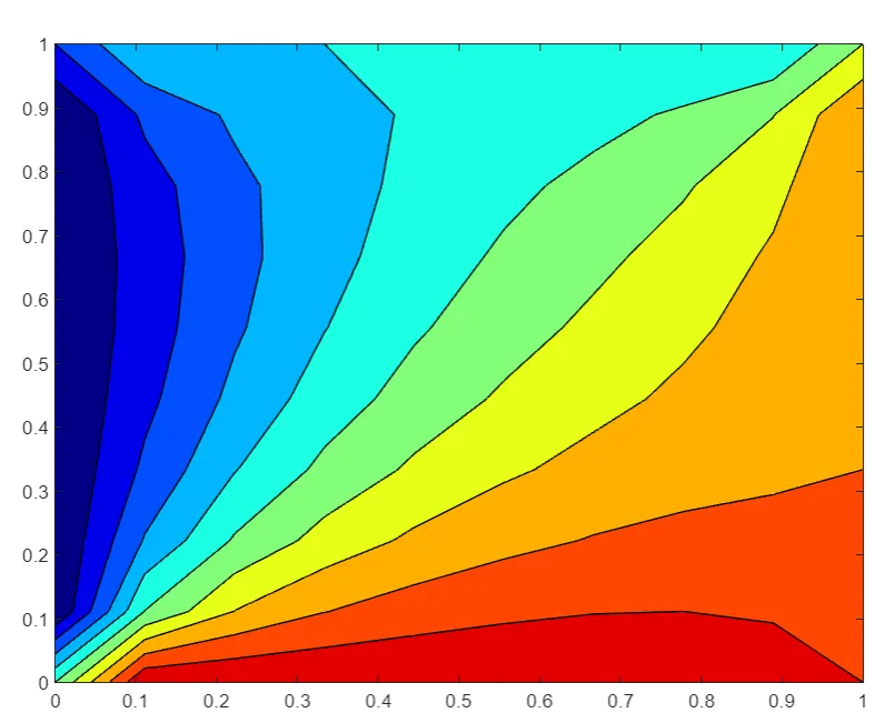
| Jacobi | Gauss - Seidel | Successive over relaxation | |
| Steady state analysis - Iterations | 208 | 112 | 75 |
| Transient Implicit scheme for 500 time steps - error | 4.1620e-8 | 4.4379e-9 | 2.7114e-10 |
CONCLUSION
- Successive over relaxtion is clearly superior, since they drastically reduce the number of iterations and if the optimum relaxation parameter is known, the computational time would also reduce significantly.
- A good guess on the initial data required to start the solution reduces the number of iterations.