Week 5.1 - Mid term project - Solving the steady and unsteady 2D heat conduction problem
1) Steady State Solution (Implicit technique):
- Jacobi Method.
- Gauss Siedel Method.
- Successive Overrelaxation Method.
2) Transient State Solution:
- Explicit Method.
- Matrix Inversion(Implicit).
clear all
close all
clc

%No_of_Nodes
nx=100;
ny=100;

%Solving the steady and unsteady 2D heat conduction problem
x=linspace(0,1,nx);
y=linspace(0,1,ny);

%Descretize Length
dx=x(2)-x(1);
dy=y(2)-y(1);

[xx,yy] = meshgrid(x,y);

%Time_Steps
t=5;
dt=1e-3;

%Initial Temperatures
T=300*ones(nx,ny);
%Boundary_Conditions
%Bottom Boundary
T(end,1:end)= 900 %_K
%Top Boundary
T(1,1:end)= 600; %_K
%Left Boundary
T(1:end,1)= 400 %_K
%Right Boundary
T(1:end,end)= 800 %_K

%Average of T at corner boundaries
T(1,1)=500;
T(end,1)=650;
T(1,end)=700;
T(end, end)=850;

%Error
error=9e9;
tolerance=1e-5;

%CFL No:-
alpha=1.4;
k=(2*(dx^2+dy^2)/(dx^2*dy^2));

%Reallocation_of_Values
Told=T;
iter1=1;
method = input('Which method?');
if(method==1)%_JACOBI_%

    tic;

    %Convergrnce Loop
    while (error>tolerance)
        for i=2:nx-1
            for j=2:ny-1

                H=(Told(i-1,j)+Told(i+1,j))/dx^2;
                V=(Told(i,j-1)+Told(i,j+1))/dy^2;
                T(i,j)=(H+V)/k;
            end
        end
        time=toc;
        %tic works with the toc function to measure elapsed time.
        % The tic function records the current time, and the toc function
        % uses the recorded value to calculate the elapsed time.

        error=max(max(abs(Told-T)));
        %Only max gets the max values from the column
        %max(max())-gives the greatest no. value

        Told=T;
        iter1=iter1+1;


    end


elseif(method==2)%_GAUSS-SEIDEL_%

    tic;

    %Convergrnce Loop
    while (error>tolerance)
        for i=2:nx-1
            for j=2:ny-1

                H=(T(i-1,j)+Told(i+1,j))/dx^2;
                V=(T(i,j-1)+Told(i,j+1))/dy^2;
                T(i,j)=(H+V)/k;
            end
        end
        time=toc;
        %tic works with the toc function to measure elapsed time.
        % The tic function records the current time, and the toc function
        % uses the recorded value to calculate the elapsed time.

        error=max(max(abs(Told-T)));
        %Only max gets the max values from the column
        %max(max())-gives the greatest no. value

        Told=T;
        iter1=iter1+1;


    end

else     %_SOR_%

    omega=1.2;

    tic;

    %Convergrnce Loop
    while (error>tolerance)
        for i = 2:nx-1
            for j = 2:ny-1
            term1 = (Told(i+1,j)+T(i-1,j))/dx^2;
            term2 = (Told(i,j+1)+T(i,j-1))/dy^2;
            T(i,j) = ((1-omega)*Told(i,j))+(omega*((term1+term2)/k));
            end
        end
        time=toc;
        %tic works with the toc function to measure elapsed time.
        % The tic function records the current time, and the toc function
        % uses the recorded value to calculate the elapsed time.

        error=max(max(abs(Told-T)));
        %Only max gets the max values from the column
        %max(max())-gives the greatest no. value

        Told=T;
        iter1=iter1+1;


    end


end

        [x,y]= contourf(xx,yy,T);
        colormap(jet)
        colorbar
        clabel(x,y)
        set(gca, 'YDir','reverse')
        pause(0.03)
        title_text1 = sprintf('Steady state Reasult = %d', iter1);
        title_text2 = sprintf('Simulation time +%f s', time);
        title_text3 = sprintf('Final error = %f', error);
        title({title_text1; title_text2; title_text3})
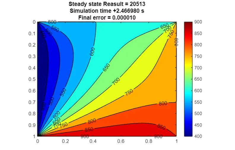
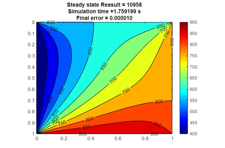
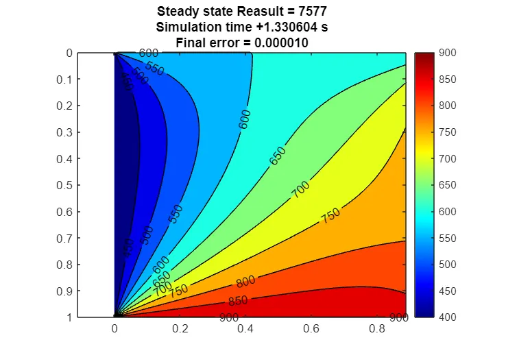
RESULTS:-
JACOBI
GAUSS-SEIDEL
SOR
2) Transient State Solution:-
- Explicit Method.
clear all
close all
clc

%No_of_Nodes
nx=100;
ny=100;

%Solving the steady and unsteady 2D heat conduction problem
x=linspace(0,1,nx);
y=linspace(0,1,ny);

%Descretize Length
dx=x(2)-x(1);
dy=y(2)-y(1);

[xx,yy] = meshgrid(x,y);

%Time Parameters
t_steps=1400;
alpha=0.001;
omega=1.2;
dt=0.01;

%CFL for X & Y directions
k1=(alpha*dt)/dx^2;
k2=(alpha*dt)/dy^2;

%Global CFL
k=k1+k2;

%Initial Temperatures
T=300*ones(nx,ny);
%Boundary_Conditions
%Bottom Boundary
T(end,1:end)= 900 %_K
%Top Boundary
T(1,1:end)= 600; %_K
%Left Boundary
T(1:end,1)= 400 %_K
%Right Boundary
T(1:end,end)= 800 %_K

%Average of T at corner boundaries
T(1,1)=500;
T(end,1)=650;
T(1,end)=700;
T(end, end)=850;

%Error
error=9;
tolerance=1e-4;


%Reallocation_of_Values
Told=T;
iter1=1;

    tic;
for i=1:1:t_steps
    %Convergrnce Loop
    while (error>tolerance)
        for i=2:nx-1
            for j=2:ny-1

                T(i,j)=Told(i,j)+k1*(Told(i-1,j)+Told(i+1,j)-2*Told(i,j))+k2*(Told(i,j-1)+Told(i,j+1)-2*Told(i,j));
            end
        end

        %tic works with the toc function to measure elapsed time.
        % The tic function records the current time, and the toc function
        % uses the recorded value to calculate the elapsed time.

        error=max(max(abs(Told-T)));
        %Only max gets the max values from the column
        %max(max())-gives the greatest no. value

        Told=T;
        iter1=iter1+1;


    end

end
        time=toc;
        figure(1)
        [x,y]= contourf(xx,yy,T);
        colormap(jet)
        colorbar
        clabel(x,y)
        set(gca, 'YDir','reverse')
        pause(0.03)
        title_text1 = sprintf('Unsteady state Explicit Result = %d', iter1);
        title_text2 = sprintf('Simulation time +%f s', time);
        title_text3 = sprintf('Final error = %f', error);
        title({title_text1; title_text2; title_text3})
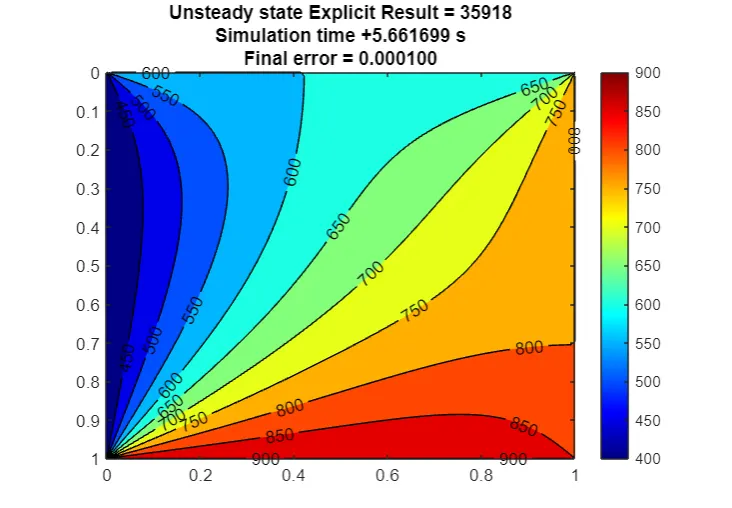
RESULT:-
B). Matrix Inversion(Implicit):-
clear all
close all
clc

% Input
nx = 100;              % Number of Nodes in X direction
ny = 100;              % Number of Nodes in Y direction
dt = 0.01;             % Time Step
alpha = 0.3;           % Thermal Diffusivity
nt = 300;              % Number of time steps

% Defining Initial Conditions -
T = 300*ones(nx,ny);   % Temperature Initial Guess

for i = 1:nx
    T(1,i) = 600;      % Top Boundary
    T(ny,i) = 900;     % Bottom Boundary
end

for j = 1:ny
    T(j,1) = 400;      % Left Boundary
    T(j,nx) = 800;     % Right Boundary
end

% Corner Nodes - Boundary Conditions
T(1,1) = (T(1,2) + T(2,1))/2;
T(1,nx) = (T(1,nx-1) + T(2,nx))/2;
T(ny,1) = (T(ny-1,1) + T(ny,2))/2;
T(ny,nx) = (T(ny,nx-1) + T(ny-1,nx))/2;

% To create 2D Mesh
x = linspace(0,1,nx);
y = linspace(0,1,ny);
dx = x(2) - x(1);
dy = y(2) - y(1);

T_old=T;             % told = t
T_prev_dt = T_old;   % tprev_dt = told
tol = 1e-4;

k1 = alpha*dt/(dx^2);
k2 = alpha*dt/(dy^2);


method = input('Iterative method = '); %iterative method selection

%JACOBI ITERATIVE METHOD
if (method==1)
    tic;
    jacobi = 1;
    for z = 1:nt
        error = 9e9;
        while(error>tol)
            for i = 2:nx-1
                for j = 2:ny-1
                    term_1 = (1 + (2*k1) + (2*k2))^-1;
                    term_2 = k1*term_1;
                    term_3 = k2*term_1;

                    H = (T_old(i-1,j) + T_old(i+1,j));
                    V = (T_old(i,j-1) + T_old(i,j+1));

                    T(i,j) = (T_prev_dt(i,j)*term_1) + (H*term_2) + (V*term_3);
                 end
            end
        error = max(max(abs(T-T_old)));
        T_old = T;
        jacobi = jacobi+1;
        end
        T_prev_dt = T;
    end
    time_taken = toc;

% Plot

figure(1)
colormap(jet);
A = contourf(x,y,T);
clabel(A);
set(gca,'YDir','reverse');
xlabel('X')
ylabel('Y')
text1 = sprintf('Number of Iteration = %d', jacobi);
text2 = sprintf('Simulation Time = %f', time_taken);
title({'Steady State Heat Condustion profile by Jacobi'; text1; text2});

end

%GAUSS-SEIDAL ITERATIVE METHOD
if (method==2)
    tic;
    gauss = 1;
    for z = 1:nt
        error = 9e9;
        while(error>tol)
            for i = 2:nx-1
                for j = 2:ny-1
                    term_1 = (1 + (2*k1) + (2*k2))^-1;
                    term_2 = k1*term_1;
                    term_3 = k2*term_1;

                    H = (T(i-1,j) + T_old(i+1,j));
                    V = (T_old(i,j+1) + T(i,j-1));

                    T(i,j) = (T_prev_dt(i,j)*term_1) + (H*term_2) + (V*term_3);
                 end
            end
        error = max(max(abs(T-T_old)));
        T_old = T;
        gauss = gauss+1;
        end
        T_prev_dt = T;
    end
    time_taken = toc;

% Plot

    figure(1)
colormap(jet);
A = contourf(x,y,T);
clabel(A);
set(gca,'YDir','reverse');
xlabel('X')
ylabel('Y')
text1 = sprintf('Number of Iteration = %d', gauss);
text2 = sprintf('Simulation Time = %f', time_taken);
title({'Unsteady State Heat Condustion Profile by Gauss-Seidal'; text1; text2});

end


%SOR ITERATIVE METHOD

if (method==3)
    tic;
    sor = 1;
    omega = 1.2;      % Over Relaxation Factor
    for z = 1:nt
        error = 9e9;
        while(error>tol)
            for i = 2:nx-1
                for j = 2:ny-1
                    term_1 = (1 + (2*k1) + (2*k2))^-1;
                    term_2 = k1*term_1;
                    term_3 = k2*term_1;

                    H = (T(i-1,j) + T_old(i+1,j));
                    V = (T_old(i,j+1) + T(i,j-1));
                    TGS = (T_prev_dt(i,j)*term_1) + (H*term_2) + (V*term_3);

                    T(i,j) = (((1-omega)*T_old(i,j)) + (omega*TGS));
                 end
            end
        error = max(max(abs(T-T_old)));
        T_old = T;
        sor = sor+1;
        end
        T_prev_dt = T;
    end
    time_taken = toc;

    % Plot

figure(1)
colormap(jet);
A = contourf(x,y,T);
clabel(A);
set(gca,'YDir','reverse');
xlabel('X')
ylabel('Y')
text1 = sprintf('Number of Iteration = %d', sor);
text2 = sprintf('Simulation Time = %f', time_taken);
title({'Unsteady State Heat Condustion Profile by SOR'; text1; text2});

end
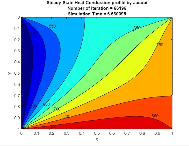
1) JACOBI METHOD:-
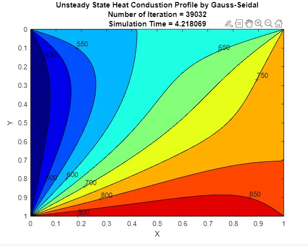
2) GAUSS-SEIDEL METHOD:-
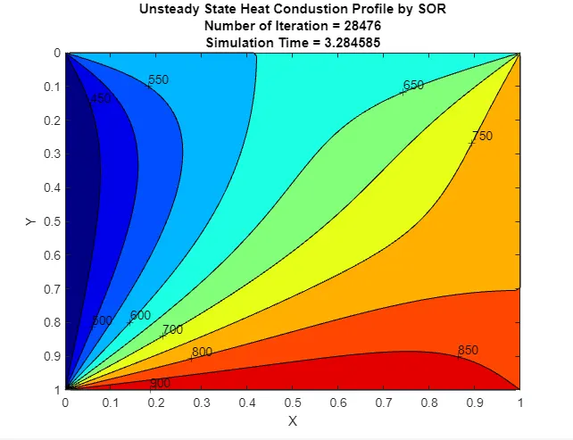
3) SOR METHOD:-
-
Jacobi method: In the Jacobi method, each component of the solution vector is updated independently based on the previous iteration's values. In other words, the updated values for each component are based on the previous iteration's values for all the other components. This method is easy to implement but can be slow to converge, especially for large systems of equations.
-
Gauss-Seidel method: In the Gauss-Seidel method, each component of the solution vector is updated based on the previous iteration's values, with the updated values being used immediately in the same iteration. This method can converge faster than the Jacobi method but may not converge for some systems of equations.
-
Successive Over-Relaxation (SOR) method: The SOR method is similar to the Gauss-Seidel method but adds a relaxation factor to accelerate convergence. The relaxation factor is a parameter that controls the amount of over-relaxation or under-relaxation of the update. The SOR method can converge faster than the Gauss-Seidel method but may require more computational resources.