Challenge

Week 5.1 - Mid term project - Solving the steady and unsteady 2D heat conduction problem

AAchutya Kumar Behera3 Feb 2023

Objective

Steady state analysis & Transient State Analysis

Solve the 2D heat conduction equation by using the point iterative techniques that were taught in the class. The Boundary conditions for the problem are as follows;

Top Boundary = 600 K

Bottom Boundary = 900 K

Left Boundary = 400 K

Right Boundary = 800 K

You will implement the following methods for solving implicit equations.

Jacobi
Gauss-seidel
Successive over-relaxation

Your absolute error criteria is 1e-4

Solution

Here, we'll learn about the 2D heat conduction equation's steady-state and transient flow concepts. Before moving on to the coding phase, we must comprehend the derivation phase when the words are discretized consecutively. Before going through it, there are a few things to keep in mind. For steady-state, we must use iterative solvers, and for transient, we must solve both the implicit and explicit schemes from the previous part.

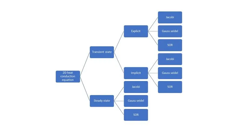
Now we are going to understand the derivation part of the steady-state condition.

Solving this by

1. Jacobi

2. Gauss-seidel

3. Successive Over Relaxation SOR

For steady-state

since d2t/dx2 + d2T/dy2 = 0, its has elliptic nature properties which we an discretize them using central differencing scheme

`(del^2T)/(delx^2)+(del^2T)/(dely^2)=0`

`(T_L-2T_P+T_R)/(Deltax^2)+(T_T-2T_P+T_B)/(Deltay^2)=0`

`(2T_P)/(Deltax^2)+(2T_P)/(Deltay^2)=(T_L+T_R)/(Deltax^2)+(T_T+T_B)/(Deltay^2)`

`T_P(2((Deltax^2+Deltay^2)/(Deltax^2Deltay^2)))=(T_L+T_R)/(Deltax^2)+(T_T+T_B)/(Deltay^2)`

we can assume

`2((Deltax^2+Deltay^2)/(Deltax^2Deltay^2))=K`

`T_P=1/K((T_L+T_R)/(Deltax^2)+(T_T+T_B)/(Deltay^2))`

In the jacobi method we use `T_L` and `T_B` will be the old value

But in GS method we use `T_L` and `T_B` will be the new value

Program of steady state 2D heat conduction equation.

% steady state 2D heat conduction equation
clear all
close all
clc

% initial condition
% L = 1
nx = 20;
ny = 20;
x = linspace(0,1,nx);
y = linspace(0,1,ny);
dx = x(2) - x(1);
dy = y(2) - y(1);

% Boundary condition
t = 300*ones(nx,ny);
t(:,1) = 400;
t(1,:) = 600;
t(:,nx) = 800;
t(ny,:) = 900;

% define temperature at the cornor
t(1,1) = 500;
t(1,ny) = 700;
t(nx,1) = 650;
t(nx,ny) = 850;

dt = 1e-2; %time step
told = t;

error = 100;
tol = 1e-4;
k = 2*(dx^2+dy^2)/(dx^2*dy^2);
method = input('Iterative method = ');

%jacobi iterative method
if (method==1)
    tic;
    jacobi = 1;
    while(error>tol)
        for i = 2:(nx-1)
            for j = 2:(ny-1)
                t(i,j) = (((told(i-1,j)+told(i+1,j))/(dx^2))+((told(i,j+1)+told(i,j-1))/(dy^2)))/k;
            end
        end
        error = max(max(abs(t-told)));
        told = t;
        jacobi = jacobi+1;
        time_taken = toc;
    end
    %plotting    
    figure(1)
    contourf(x,y,t,'ShowText','on');
    colormap(jet);
    colorbar;
    xlabel('X')
    ylabel('Y')
    text1 = sprintf('number of iteration = %d', jacobi);
    text2 = sprintf('simulation time = %f', time_taken);
    title({'Steady state heat condustion profile by jacobi'; text1; text2});
end

% Gauss seidel iterative method

if (method==2)
    tic;
    gs = 1;
    while(error>tol)
        for i = 2:(nx-1)
            for j = 2:(ny-1)
                t(i,j) = (((t(i-1,j)+told(i+1,j))/(dx^2))+((told(i,j+1)+t(i,j-1))/(dy^2)))/k;
            end
        end
        error = max(max(abs(t-told)));
        told = t;
        gs = gs+1;
        time_taken = toc;
    end
    %plotting    
    figure(2)
    contourf(x,y,t,'ShowText','on');
    colormap(jet);
    colorbar;
    xlabel('X')
    ylabel('Y')
    text1 = sprintf('number of iteration = %d', gs);
    text2 = sprintf('simulation time = %f', time_taken);
    title({'Steady state heat condustion profile by gaues seidel'; text1; text2});
end

% SOR iterative method
if (method==3)
    tic;
    sor = 1;
    omega = 1.4; %over relaxation factor
    while(error>tol)
        for i = 2:(nx-1)
            for j = 2:(ny-1)
                term1 =(t(i-1,j)+told(i+1,j))/(dx^2);
                term2 =(told(i,j+1)+t(i,j-1))/(dy^2);
                t(i,j) = ((told(i,j)*(1-omega)))+(omega*(term1+term2))/k;
            end
        end
        error = max(max(abs(t-told)));
        told = t;
        sor = sor+1;
        time_taken = toc;
    end
    %plotting    
    figure(3)
    contourf(x,y,t,'ShowText','on');
    colormap(jet);
    colorbar;
    xlabel('X')
    ylabel('Y')
    text1 = sprintf('number of iteration = %d', sor);
    text2 = sprintf('simulation time = %f', time_taken);
    title({'Steady state heat condustion profile by successive over relaxation'; text1; text2});
end

Results

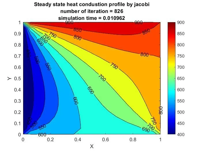
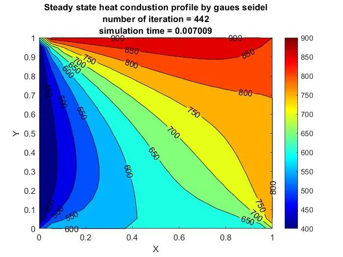
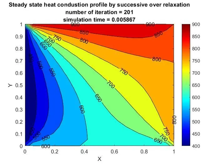
From the data above, it is clear that the SOR approach performs better in terms of the number of simulations performed and the number of iterations.

Transient (Unsteady) state simulation:

We'll now focus on implicit and explicit approaches in the modelling of the transient state.

1. Implicit schemes

2. Explicit schemes

In order to produce numerical approximations to the solutions of time-dependent ordinary and PDEs, which is necessary in computer simulations of physical processes, explicit and implicit techniques are methodologies used in numerical analysis. While implicit techniques arrive at a solution by solving an equation involving both the present state of the system and the later one, explicit methods determine the state of a system at a later time from the state of the system at the current time.

Mathematically, if

the current system state is `Y(t)`

state at the later time is `Y(t+Deltat)`

small time step is `Deltat`

then, for an explicit method `Y(t+Deltat)=f(Y(T))`

while for an implicit method `g(Y(t),Y(t+Deltat))=0`

Derivation

Applying the 2D transient heat conduction equation

`(delT)/(delt)+alpha((del^2T)/(delx^2)+(del^2T)/(dely^2))=0`

After discretize the equation

`(T_P^(n+1)-T_P^n)/(Deltat)+alpha((T_R-2T_P+T_L)/(Deltax^2)+(T_T-2T_P+T_B)/(Deltay^2))=0`

`T_P^(n+1)=T_P^n+alphaDeltat((T_R-2T_P+T_L)/(Deltax^2)+(T_T-2T_P+T_B)/(Deltay^2))`

For explicit scheme

`T_P^(n+1)=1/(1+2K_1+2K_2)(T_P^n+K_1(T_L+T_R)^n+K_2(T_T+T_B)^n)`

For implicit scheme

`T_P^(n+1)=1/(1+2K_1+2K_2)(T_P^n+K_1(T_L+T_R)^(n+1)+K_2(T_T+T_B)^(n+1))`

Programming for Transient State Implicitly

% transient state 2D heat conduction equation
clear all
close all
clc

% initial condition
% L = 1
nx = 20;
ny = 20;
x = linspace(0,1,nx);
y = linspace(0,1,ny);
dx = x(2) - x(1);
dy = y(2) - y(1);

% Boundary condition
t = 300*ones(nx,ny);
t(:,1) = 400;
t(1,:) = 600;
t(:,nx) = 800;
t(ny,:) = 900;

% define temperature at the cornor
t(1,1) = 500;
t(1,ny) = 700;
t(nx,1) = 650;
t(nx,ny) = 850;

nt = 300; % No.of steps

dt = 1e-2; %time step
told = t;
tprev_dt = told;

error = 100;
tol = 1e-4;
alpha = 0.3; % Thermal diffusivity
k1 = alpha*dt/(dx^2);
k2 = alpha*dt/(dy^2);

method = input('Iterative method = ');

% jacobi method
if (method==1)
    tic;
    jacobi = 1;
    for p = 1:nt
        error =100;
        while(error>tol)
            for i = 2:(nx-1)
                for j = 2:(ny-1)
                    term1 = (1+(2*k1)+(2*k2))^-1;
                    term2 = k1*term1;
                    term3 = k2*term1;
                    h = (told(i-1,j)+told(i+1,j));
                    v = (told(i,j+1)+told(i,j-1));
                    t(i,j) = ((tprev_dt(i,j)*term1)+(h*term2)+(v*term3));
                end
            end
        
            error = max(max(abs(t-told)));
            told = t;
            jacobi = jacobi+1;
         end
         tprev_dt = t ;
    end
    time_taken = toc;

%plotting    
figure(1)
contourf(x,y,t,'ShowText','on');
colormap(jet);
colorbar;
xlabel('X')
ylabel('Y')
text1 = sprintf('number of iteration = %d', jacobi);
text2 = sprintf('simulation time = %f', time_taken);
title({'Transient state heat conduction profile Implicit-Jacobi'; text1; text2});
end

% gauss seidel method
if (method==2)
    tic;
    gauss = 1;
    for p = 1:nt
        error =100;
        while(error>tol)
            for i = 2:(nx-1)
                for j = 2:(ny-1)
                    term1 = (1+(2*k1)+(2*k2))^-1;
                    term2 = k1*term1;
                    term3 = k2*term1;
                    h = (t(i-1,j)+told(i+1,j));
                    v = (told(i,j+1)+t(i,j-1));
                    t(i,j) = ((tprev_dt(i,j)*term1)+(h*term2)+(v*term3));
                end
            end
        
            error = max(max(abs(t-told)));
            told = t;
            gauss = gauss+1;
         end
         tprev_dt = t; 
    end
    time_taken = toc;

    %plotting    
    figure(1)
    contourf(x,y,t,'ShowText','on');
    colormap(jet);
    colorbar;
    xlabel('X')
    ylabel('Y')
    text1 = sprintf('number of iteration = %d', gauss);
    text2 = sprintf('simulation time = %f', time_taken);
    title({'Transient state heat conduction profile Implicit-Gauss-seidel'; text1; text2});
end

% successive over relaxation method


if (method==3)
    tic;
    sor = 1;
    omega = 1.2; % Over relaxation factor
    for p = 1:nt
        error =100;
        while(error>tol)
            for i = 2:(nx-1)
                for j = 2:(ny-1)
                    term1 = (1+(2*k1)+(2*k2))^-1;
                    term2 = k1*term1;
                    term3 = k2*term1;
                    h = (t(i-1,j)+told(i+1,j));
                    v = (told(i,j+1)+t(i,j-1));
                    t(i,j) = (told(i,j)*(1-omega))+(omega*((tprev_dt(i,j)*term1)+(h*term2)+(v*term3)));
                end
            end
        
            error = max(max(abs(t-told)));
            told = t;
            sor = sor+1;
         end
         tprev_dt = t ;
    end
    time_taken = toc;

%plotting    
figure(1)
contourf(x,y,t,'ShowText','on');
colormap(jet);
colorbar;
xlabel('X')
ylabel('Y')
text1 = sprintf('number of iteration = %d', sor);
text2 = sprintf('simulation time = %f', time_taken);
title({'Transient state heat conduction profile Implicit-SOR'; text1; text2});
end

Results

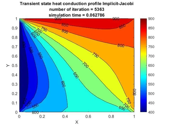
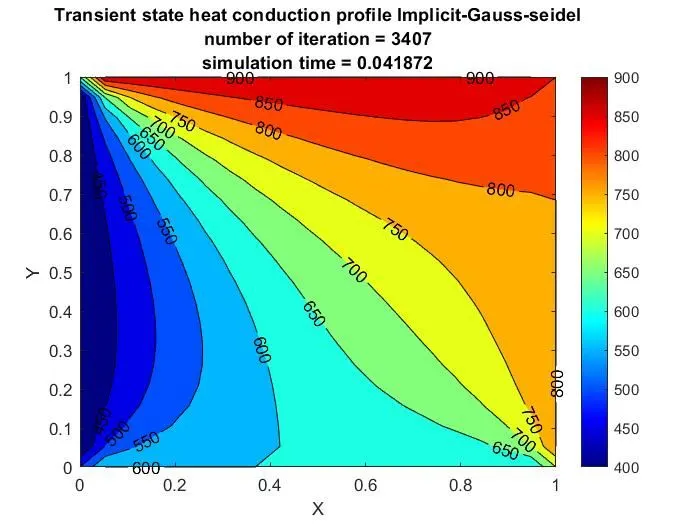
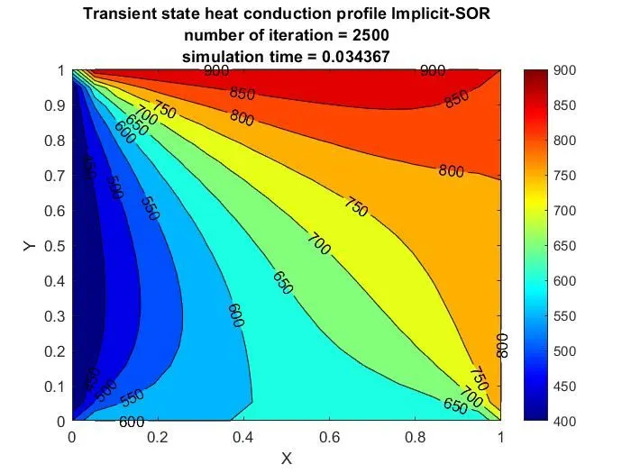
The conclusion of the research exists is identical to that of the steady state, and it has been shown that SOR approaches perform better when there are fewer simulations and less run time.

Programming for transient explicit scheme

% Solving Steady and Transient 2D heat conduction problem
% Transient state solution with EXPLICIT


clear all
close all
clc

%initial conditions
%L = 1
nx = 10;
ny = 10;
nt = 300; % No.of steps
x = linspace(0,1,nx);
y = linspace(0,1,ny);
dx = x(2) - x(1);
dy = y(2) - y(1);

% initial temp condition

t = 300*ones(nx,ny);  
t(:,1) = 400;
t(1,:) = 600;
t(:,ny) = 800;
t(nx,:) = 900;

% defining the temperature at corner points

t(1,1) = 500;
t(nx,ny) = 850;
t(1,ny) = 700;
t(nx,1) = 650;

dt = 0.01; %time step
told=t;
alpha = 0.3; % Thermal diffusivity

k1 = (alpha*dt)/(dx^2);
k2 = (alpha*dt)/(dy^2);
CFL = alpha*dt/(dx^2);

%EXPLICIT METHOD
% running for loop

tic;
explicit = 1;
for p = 1:nt
    for i = 2:(nx-1)
        for j = 2:(ny-1)
            term1 = (told(i-1,j)-2*told(i,j)+told(i+1,j));
            term2 = (told(i,j-1)-2*told(i,j)+told(i,j+1));
            t(i,j) = ((told(i,j))+(k1*term1)+(k2*term2));
        end
    end
        
    told = t;
    explicit = explicit+1;
end

time_taken = toc;
  
%Plotting   
figure(1)
contourf(x,y,t,'ShowText','on');
colormap(jet);
colorbar;
xlabel('X')
ylabel('Y')
text1 = sprintf('timen = %d', dt*nt);
text2 = sprintf('simulation time = %f', time_taken);
title({'Transient state heat conduction profile Explicit'; text1; text2});

Result

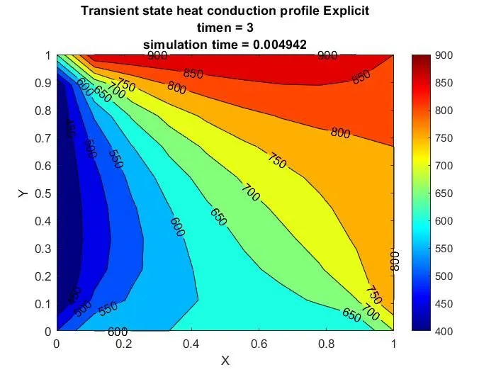
The above simulation shows that explicit techniques converge more quickly than implicit approaches, which need less time for simulations. We may use the SOR approach since it converges quicker than any other method for a steady state.

Explicit approaches provide a higher degree of accuracy and need less time to run.

Week 5.1 - Mid term project - Solving the steady and unsteady 2D heat conduction problem

Ship work like this
in your own course.

Talk to a career counsellor

Ship work like thisin your own course.

Talk to a career counsellor

Ship work like this
in your own course.