Week 5.1 - Mid term project - Solving the steady and unsteady 2D heat conduction problem

AIM

Solve the 2D heat conduction equation by using the point iterative techniques that were taught in the class. The Boundary conditions for the problem are as follows;

Top Boundary = 600 K

Bottom Boundary = 900 K

Left Boundary = 400 K

Right Boundary = 800 K

You will implement the following methods for solving implicit equations.

• Jacobi
• Gauss-seidel
• Successive over-relaxation

Your absolute error criteria is 1e-4.

You will write code for both implicit and explicit schemes (This is for the transient analysis only)

THEORY

The Heat conduction equation is defined by a partial differential equation(PDE) given by-

This equation tells about the heeat behaviour and distribution with respect to change in time.

where T is the temperature, α is thermal diffusivity and (x,y,z,t) are space and time variables respectively.

Descritization:

We have 3 types of discritization:-

1) Central differencing

2) Forward differencing

3) Backward differencing

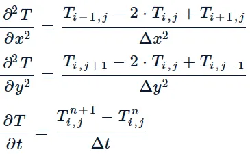
Here, for our second-order partial differential equation of T w.r.t x and y we will use Central differencing as it elliptical or we can say it takes information from all direction in the mesh. For discretize our time derivative term of T w.r.t t we will use Forward differencing method as it is hyperbolic or we can say it takes information from left to right.

Let T_i,j be the temperature at the point of intersection of i^th row and j^th column in the assumed square field. The above PDE can be discretized as follows

First let's define what are the iterative techniques we are using here:

The Descritized form for steady state conduction is represented as-

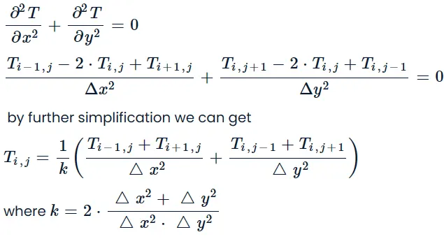
The above eqn will help us to tell the temperature values at all nodes defined by us as a function of the temperature of its neighboring nodes.

This above equation is to be solved by fixed point method which is solved with help of iterative solvers like:-

1)Jacobi

2)Gauss-Siedel

3)Successive Over Relaxation (SOR)

1. Jacobi

In this method, the values of T^(n+1) iteration is calculated with the help of old values of T at nth iteration and repeated until we obtain a converged solution for T.

This method is also called the method of simultaneous displacements as all values at nth iteration are updated with the values at (n+1) iteration simultaneously for each iterations.

2. Gauss-seidel

In this iteration we assume the values obtained in Jacobi iteration for the next equation immediately without waiting for completion of first cycle.

3. Successive Over-relaxation (SOR)

This method is an updated version of previous two. In addition we use the relaxation factor to ease the process. For this analysis we use the relaxation facor to be greater than 1 and less than 2.

MATLAB CODE

1) Steady state analysis

clear all
close all
clc

% Definig the 2D grid
nx = 15;
ny = 15;

% Giving intervals
x = linspace(0,1,nx);
y = linspace(0,1,ny);

% Defining element dx and dy size
dx = x(2) - x(1);
dy = y(2) - y(1);

% Defining gridspace
[xx yy] = meshgrid(x,y);

% providing the initial conditions
t = 200*ones(nx,ny); % 200 is random 
% providing the boundary conditions
t(1,:) = 600; % top
t(ny,:) = 900; % bottom
t(:,1) = 400; % left
t(:,nx) = 800; % right

% define constant to simplify procedure
k = (2*(dx^2+dy^2)/(dx^2*dy^2));
t_old = t;
t_p = t;

% Creating comparision parameters
threshold = 0.0001;
error = 1000;

% creating input choice for solver
Solver = input('Which Solver?')
% 1 = Jacobi; 2 = Gauss- Siedal; 3 = SOR

% Creating Jacobi solver
if Solver ==1
    tic;
    iteration_j = 1; % Initializing 1st iteration

    while error>threshold  % Loop for convergence
        for i = 2:nx-1 % Loop for space term (rows)
            for j = 2:ny-1 % Loop for space term (column)
                L = t_old(i-1,j);
                R = t_old(i+1,j);
                B = t_old(i,j-1);
                T = t_old(i,j+1);
                
                H= (L +R)/dx^2;
                V = (B + T)/dy^2;
                
                t(i,j) = (H +V)/k;
            end
        end
        time_j = toc;
        iteration_j = iteration_j + 1;
        error = max(max(abs(t-t_old)));
        t_old = t;
    
        contourf(xx,yy,t,ShowText="on")
        set(gca,'YDir','reverse') % Command to reverse the Y cordinates
        title_text1 = sprintf('Iterations to reach staedy state(javobi) = %d', iteration_j);
        title_text2 = sprintf('Simulation time  +%f s', time_j);
        title_text3 = sprintf('Max error %g ', error);
        title({title_text1; title_text2; title_text3})
        colormap (jet) 
        colorbar
       
       
    end
end

% Setting up for Gauss-Siedal
if Solver == 2
 tic;
    iteration_j = 1; % Initializing 1st iteration

    while error>threshold  % Loop for convergence
        for i = 2:nx-1 % Loop for space term (rows)
            for j = 2:ny-1 % Loop for space term (column)
                R = t_old(i+1,j);
                T = t_old(i,j+1);
                
                H= (t(i-1,j) + R)/dx^2;
                V= (t(i,j-1) + T)/dy^2;
                
                t(i,j) = (H +V)/k;
            end
        end
        time_j = toc;
        iteration_j = iteration_j + 1;
        error = max(t-t_old);
        t_old = t;
    
        contourf(xx,yy,t,ShowText="on")
        set(gca,'YDir','reverse') % Command to reverse the Y cordinates
        title_text1 = sprintf('Iterations to reach staedy-state(Gauss) = %d', iteration_j);
        title_text2 = sprintf('Simulation time  +%f s', time_j);
        title_text3 = sprintf('Max error %g ', error);
        title({title_text1; title_text2; title_text3})
        colormap (jet) 
        colorbar
       
       
    end
end

% Setting up for SOR method
alpha = 0.5;   % thermal diffusivity
omega = 1.5;   % SOR value, random number b/w 1-2
if Solver == 3
    tic;
    iteration_j = 1; % Initializing 1st iteration

    while error>threshold  % Loop for convergence
        for i = 2:nx-1 % Loop for space term (rows)
            for j = 2:ny-1 % Loop for space term (column)
                R = t_old(i+1,j);
                T = t_old(i,j+1);
                
                H= (t(i-1,j) + R)/dx^2;
                V= (t(i,j-1) + T)/dy^2;
                
                tgs(i,j) = (H +V)/k;
                t(i,j) = (1-omega)*(t_old(i,j))+omega*tgs(i,j);
            end
        end
        time_j = toc;
        iteration_j = iteration_j + 1;
        error = max(t-t_old);
        t_old = t;
    
        contourf(xx,yy,t,ShowText="on")
        set(gca,'YDir','reverse') % Command to reverse the Y cordinates
        title_text1 = sprintf('Iterations to reach staedy-state(SOR) = %d', iteration_j);
        title_text2 = sprintf('Simulation time  +%f s', time_j);
        title_text3 = sprintf('Max error %g ', error);
        title({title_text1; title_text2; title_text3})
        colormap(jet) 
        colorbar
       
       
    end
end

2) Implicit transient analysis

clear all
close all
clc

% Definig the 2D grid
nx = 15;
ny = 15;

% Giving random(in a range) value to constants
alpha = 0.5;   % thermal diffusivity
omega = 1.5;   % SOR value, random number b/w 1-2

% Giving intervals
x = linspace(0,1,nx);
y = linspace(0,1,ny);

% Defining element dx and dy size
dx = x(2) - x(1);
dy = y(2) - y(1);

% Devining time step dt
dt = 0.01;

% Defining gridspace
[xx yy] = meshgrid(x,y);

% providing the initial conditions
t = 200*ones(nx,ny); % 200 is random 
% providing the boundary conditions
t(1,:) = 600; % top
t(ny,:) = 900; % bottom
t(:,1) = 400; % left
t(:,nx) = 800; % right

% define constant to simplify procedure
k1= alpha*dt/dx^2;
k2= alpha*dt/dy^2;
k = 1+(2*k1)+(2*k2);
t_old = t;
t_p = t;

% Creating comparision parameters
threshold = 0.0001;
error = 1000;

% creating input choice for solver
Solver = input('Which Solver?')
% 1 = Jacobi; 2 = Gauss- Siedal; 3 = SOR

% Creating Jacobi solver
if Solver ==1
    tic;
    iteration_j = 1; % Initializing 1st iteration

    while error>threshold  % Loop for convergence
        for i = 2:nx-1 % Loop for space term (rows)
            for j = 2:ny-1 % Loop for space term (column)
                L = t_old(i-1,j);
                R = t_old(i+1,j);
                B = t_old(i,j-1);
                T = t_old(i,j+1);
                
                H= (L +R);
                V = (B + T);
                
                t(i,j) = ((t_p(i,j)+H*k1 +V*k2)/k);
            end
        end
        time_j = toc;
        iteration_j = iteration_j + 1;
        error = max(max(abs(t-t_old)));
        t_old = t;
    
        contourf(xx,yy,t,ShowText="on")
        title_text1 = sprintf('Iterations to reach staedy state(javobi) = %d', iteration_j);
        title_text2 = sprintf('Simulation time  +%f s', time_j);
        title_text3 = sprintf('Max error %g ', error);
        title({title_text1; title_text2; title_text3})
        colormap (jet) 
        colorbar
       
       
    end
end

% Setting up for Gauss-Siedal
if Solver == 2
 tic;
    iteration_j = 1; % Initializing 1st iteration

    while error>threshold  % Loop for convergence
        for i = 2:nx-1 % Loop for space term (rows)
            for j = 2:ny-1 % Loop for space term (column)
                R = t_old(i+1,j);
                T = t_old(i,j+1);
                
                H= (t(i-1,j) + R);
                V= (t(i,j-1) + T);
                
                t(i,j) = ((t_p(i,j)+H*k1 +V*k2)/k);
            end
        end
        time_j = toc;
        iteration_j = iteration_j + 1;
        error = max(max(abs(t-t_old)));
        t_old = t;
    
        contourf(xx,yy,t,ShowText="on")
        title_text1 = sprintf('Iterations to reach staedy-state(Gauss) = %d', iteration_j);
        title_text2 = sprintf('Simulation time  +%f s', time_j);
        title_text3 = sprintf('Max error %g ', error);
        title({title_text1; title_text2; title_text3})
        colormap (jet) 
        colorbar
       
       
    end
end

% Setting up for SOR method
alpha = 0.5;   % thermal diffusivity
omega = 1.5;   % SOR value, random number b/w 1-2
if Solver == 3
    tic;
    iteration_j = 1; % Initializing 1st iteration

    while error>threshold  % Loop for convergence
        for i = 2:nx-1 % Loop for space term (rows)
            for j = 2:ny-1 % Loop for space term (column)
                R = t_old(i+1,j);
                T = t_old(i,j+1);
                
                H= (t(i-1,j) + R)/dx^2;
                V= (t(i,j-1) + T)/dy^2;
                
                tgs(i,j) = (H +V)/k;
                t(i,j) = (1-omega)*(t_old(i,j))+omega*tgs(i,j);
            end
        end
        time_j = toc;
        iteration_j = iteration_j + 1;
        tgs(i,j) = ((t_p(i,j)+H*k1 +V*k2)/k);
        t(i,j) = (1-omega)*(t_old(i,j))+omega*tgs(i,j);
    
        contourf(xx,yy,t,ShowText="on")
        title_text1 = sprintf('Iterations to reach staedy-state(SOR) = %d', iteration_j);
        title_text2 = sprintf('Simulation time  +%f s', time_j);
        title_text3 = sprintf('Max error %g ', error);
        title({title_text1; title_text2; title_text3})
        colormap(jet) 
        colorbar
       
       
    end
end

3) Explicit transient analysis

clear all
close all
clc

% Definig the 2D grid
nx = 10;
ny = nx;

% Giving random(in a range) value to constants
alpha = 0.3;   % thermal diffusivity
omega = 1.2;   % SOR value, random number b/w 1-2

% Giving intervals
x = linspace(0,1,nx);
y = linspace(0,1,ny);

% Defining element dx and dy size
dx = x(2) - x(1);
dy = y(2) - y(1);

% Devining time step dt
t = 7;
dt = 0.01;
nt = t/dt;

% Defining gridspace
[xx yy] = meshgrid(x,y);

% providing the initial conditions
t = 300*ones(nx,ny); % 200 is random 
% providing the boundary conditions
t(1,:) = 600; % top
t(ny,:) = 900; % bottom
t(:,1) = 400; % left
t(:,nx) = 800; % right

% define constant to simplify procedure
k1= alpha*dt/dx^2;
k2= alpha*dt/dy^2;
k = 1-(2*k1)-(2*k2);
t_old = t;
t_p = t;

% Creating comparision parameters
threshold = 0.0001;
error = 1000;

% creating input choice for solver
Solver = input('Which Solver?')
% 1 = Jacobi; 2 = Gauss- Siedal; 3 = SOR

% Creating Jacobi solver
if Solver ==1
    tic;
    iteration_j = 1; % Initializing 1st iteration

    while error>threshold  % Loop for convergence
        for i = 2:nx-1 % Loop for space term (rows)
            for j = 2:ny-1 % Loop for space term (column)
                L = t_old(i-1,j);
                R = t_old(i+1,j);
                B = t_old(i,j-1);
                T = t_old(i,j+1);
                
                H= (L +R);
                V = (B + T);
                
                t(i,j) = t_p(i,j)*k + k1*H +k2*V;
            end
        end
        time_j = toc;
        iteration_j = iteration_j + 1;
        error = max(max(abs(t-t_old)));
        t_old = t;
    
        contourf(xx,yy,t,ShowText="on")
        title_text1 = sprintf('Iterations to reach staedy state(javobi) = %d', iteration_j);
        title_text2 = sprintf('Simulation time  +%f s', time_j);
        title_text3 = sprintf('Max error %g ', error);
        title({title_text1; title_text2; title_text3})
        colormap (jet) 
        colorbar
       
       
    end
end

% Setting up for Gauss-Siedal
if Solver == 2
 tic;
    iteration_j = 1; % Initializing 1st iteration

    while error>threshold  % Loop for convergence
        for i = 2:nx-1 % Loop for space term (rows)
            for j = 2:ny-1 % Loop for space term (column)
                R = t_old(i+1,j);
                T = t_old(i,j+1);
                
                H= (t(i-1,j) + R);
                V= (t(i,j-1) + T);
                
                t(i,j) = t_p(i,j)*k +H*k1 +V*k2;
            end
        end
        time_j = toc;
        iteration_j = iteration_j + 1;
        error = max(max(abs(t-t_old)));
        t_old = t;
    
        contourf(xx,yy,t,ShowText="on")
        title_text1 = sprintf('Iterations to reach staedy-state(Gauss) = %d', iteration_j);
        title_text2 = sprintf('Simulation time  +%f s', time_j);
        title_text3 = sprintf('Max error %g ', error);
        title({title_text1; title_text2; title_text3})
        colormap (jet) 
        colorbar
       
       
    end
end

% Setting up for SOR method
alpha = 0.5;   % thermal diffusivity
omega = 1.5;   % SOR value, random number b/w 1-2
if Solver == 3
    tic;
    iteration_j = 1; % Initializing 1st iteration

    while error>threshold  % Loop for convergence
        for i = 2:nx-1 % Loop for space term (rows)
            for j = 2:ny-1 % Loop for space term (column)
                R = t_old(i+1,j);
                T = t_old(i,j+1);
                
                H= (t(i-1,j) + R);
                V= (t(i,j-1) + T);
                
                tgs(i,j) = t_p(i,j)*k +H*k1 +V*k2;
                t(i,j) = (1-omega)*(t_old(i,j))+omega*tgs(i,j);
            end
        end
        time_j = toc;
        iteration_j = iteration_j + 1;
        tgs(i,j) = ((t_p(i,j)+H*k1 +V*k2)/k);
        t(i,j) = (1-omega)*(t_old(i,j))+omega*tgs(i,j);
    
        contourf(xx,yy,t,ShowText="on")
        title_text1 = sprintf('Iterations to reach staedy-state(SOR) = %d', iteration_j);
        title_text2 = sprintf('Simulation time  +%f s', time_j);
        title_text3 = sprintf('Max error %g ', error);
        title({title_text1; title_text2; title_text3})
        colormap(jet) 
        colorbar
       
       
    end
end

RESULTS

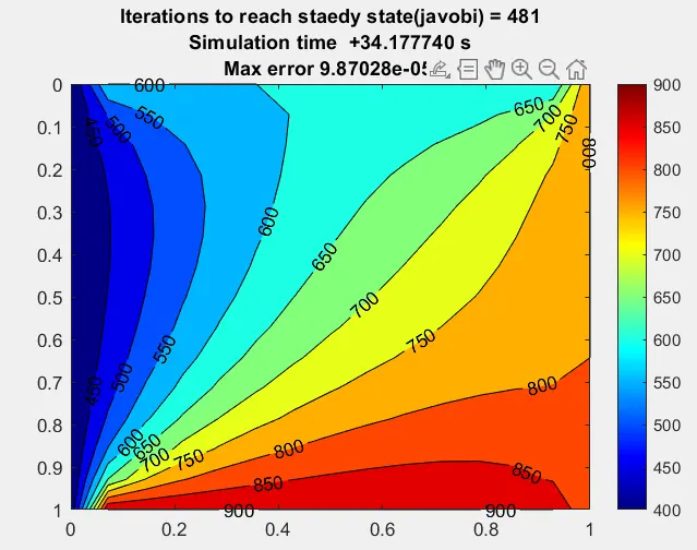
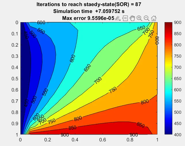
1) Steady state analysis

1.1) Jacobi

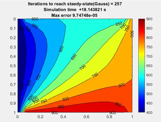
1.2) Gauss-seidel

1.3) Successive over-relaxation (SOR)

2) Implicit transient analysis

2.1) Jacobi

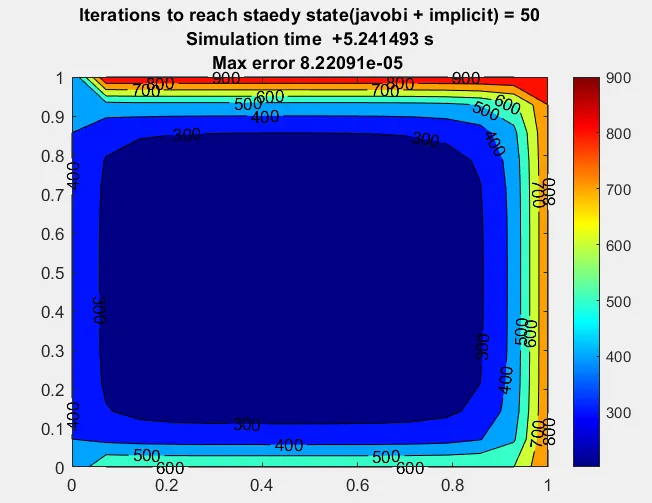
2.2) Gauss-seidel

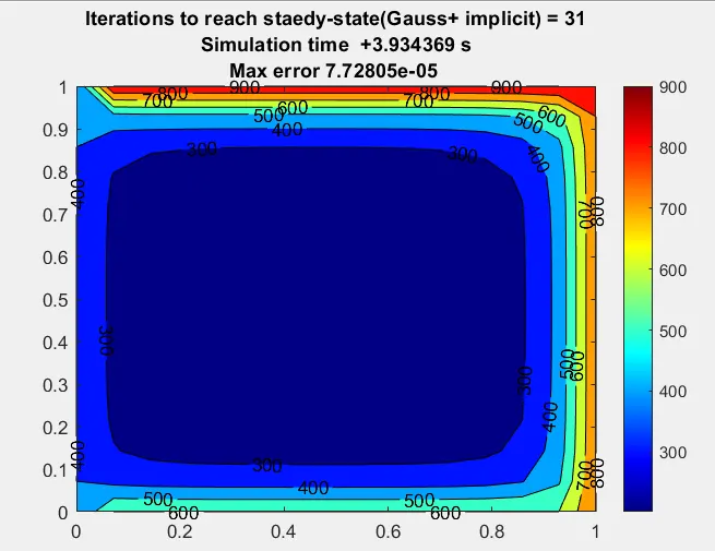
2.3) Successive over-relaxation (SOR)

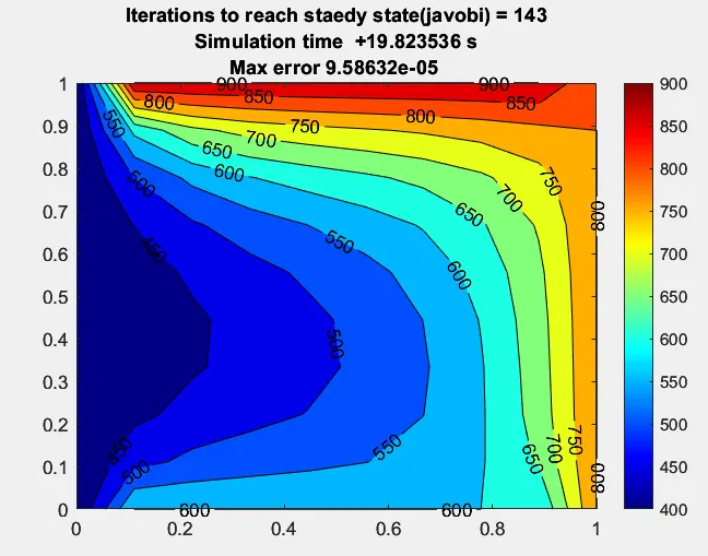
3) Explicit transient analysis

3.1) Jacobi

3.2) Gauss-seidel

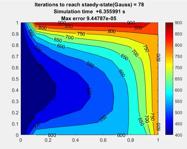
3.3) Successive over-relaxation (SOR)

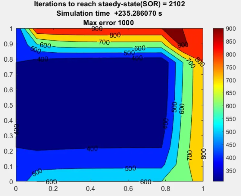
CONCLUSION

From the results obtained we can conclude the following points:-

1) Steady-state results are simplified and easy to analyse as compared to the 2 transient-state results.

2) The number of iterations as time required to reach steady state are the minimum for SOR solver as compared to others.

3) Implicit solver is almost independent of CFL number wheeareas the Explicit solver depends highly on CFL number and gives faster results for low CFL number.

4) Number of iterations depends on many factors/parameters like:-

Diffusion Constant

Number of Nodes

Scheme (explicit>implicit)