Challenge

Week 5.1 - Mid term project - Solving the steady and unsteady 2D heat conduction problem

RRuthreesh T20 Jan 2023

OBJECTIVE:

To Solve the 2D heat conduction equation by using the point iterative techniques that were taught in the class. The Boundary conditions for the problem are as follows;

Top Boundary = 600 K

Bottom Boundary = 900 K

Left Boundary = 400 K

Right Boundary = 800 K

I will be taking a 2D spacial box for the given boundary conditioned states having 300k as the initial teprature

The 2D heat equation is partial derivative and while solving for iterations , there are two sates of equation involving

STEADY STATE
UNSTEADY STATE

STEADY STATE

As the 2D heat equation is a partial derivative the equation in steady state omits the time derivative function and it goes by

`(delta^2T)/(deltax^2)+(delta^2T)/(deltay^2) = 0`
T - temperature
(x,y) - axes of the tempearature function

In this steady state the iterations used for solving the equations are as follows

jacobi
Gauss -seidel
SOR(successive over relaxation factor)

UNSTEADY STATE

unsteady state is the transient way of steady state i.e it involves time derivative as the function here depend upon the time steps corresponding the equation. The equation here goes by

`(deltaT)/(deltat)+((delta^2T)/(deltax^2)+(delta^2T)/(deltay^2)) = 0`
`(deltaT)/(deltat)` - time derivative deciding the time steps to reac steady state.

2D HEAT CONDUCTION EQUATION SOLVING (STEADY STATE);

`(delta^2T)/(deltax^2)+(delta^2T)/(deltay^2) = 0` solving this equation by central differencing

`(T{L} - 2T{P}+T{R})/(Deltax^2)+(T{T}-2T{P} +T{B})/(Deltay^2)` where

T{L} - temperature at left point
T{R} - temperature at right point
T{P} - temperature at center point

By further classification the equation becomes `T{P} = (1/K)[(T{L}-T{R})/(Deltax^2) +(T{T}-T{B})/(Deltay^2)]` where K is `(2 (Deltax^2 + Deltay^2)/(Deltax^2Deltay^2))`

with the help of the classified equation above , coding in matlab with iterative techniques converges the solution after certain iteration to get the optimised output

IMPLICIT METHOD

In implicit method the equation set for finding the solution for (n+1)th component .i.e only one known in the equation for solving remaining remains unknown

EXPICIT METHOD

In explicit method the equation is set for finding the solution for(nth) component where only there is one unknown .

JACOBI METHOD OF ITERATION

In this iterative method the new solution for the equation is taken as the reference for the next solvable equation , here T(i+1,j+1) corresponds to new solution for the equation(depending upon the formula generally taken as T(new). For the next step iteration T(new) ,T(old)(i+1,j+1) is taken as the reference and the next iterative is found out . Here in the Jacobi iterative method is considered as an iterative algorithm which is used for determining the solutions for the system of linear equations in numerical linear algebra, which is diagonally dominant.

GAUSS - SEIDAL METHOD OF ITERATION

In this iterative method , the equation which corresponds to the next solvable equation takes the reference from the latest apllied t(i,j) i.e if a solution for the upcoming next solution is not fully defined it takes the reference from the latest values available in the solution (partially referred ) . If a matrix contain n number of matrix , the sequation is conditiones to take reference from the previous temperature values then the the solver takes the reference from (i-1)th component in the matrix . By comparison it is found that the Gauss seidel requires less iteration numbers when compared to jacobi method

SOR(successive over relaxtion)

This method is used to emphasize the effieciency of jacobi and gauss seidel methods. This method can be used for both methods to reduce the iteration numbers and to converge quicker. A relaxaion factor is used to modify the equation . `omega`is called the relaxation factor and the formual goes by `(1-omega)T{old} +omega(T{g.s}`where T{g.s} is the temperature solving for the gauss seidel iteration technique.

2D HEAT EQUATION

This equation signifies how heat is diffused in a solid state moving from surface to other surface over a function of time where it moves from higher to lower or vice versa .

CODE :

STEADY STATE

JACOBI CONDITION

clear all
close all
clc


%Solving the Steady state 2D heat conduction (Jacobi Method)

%Input Parameters
%Number of grid points
nx = 10;
ny = nx;

x = linspace(0,1,nx);
y = linspace(0,1,ny);

dx = x(2) - x(1);
dy = dx;

%Absolute error criteria > tolerance
err = 9e9;
tolerance = 1e-4;

%Defining Boundary conditions
T_L = 400;
T_T = 600;
T_R = 800;
T_B = 900;

T = 300*ones(nx,ny);

T(2:ny - 1, 1)  = T_L;
T(2:ny - 1, nx) = T_R;
T(1, 2:nx - 1)  = T_T;
T(ny, 2:nx - 1) = T_B;

%Calculating Average temperature at corners
T(1,1) = (T_T + T_L)/2;
T(nx,ny) = (T_R + T_B)/2;
T(1,ny) = (T_T + T_R)/2;
T(nx,1) = (T_L + T_B)/2;

%Assigning orginal values to T
T_intial = T;
T_old = T;


%Calculation of 2D steady heat conduction EQUATION by JACOBI method
iterative_solver = 1;

if iterative_solver == 1
    jacobi_iteration = 1;
    
    while(err > tolerance)
        
        for i = 2:nx - 1
            
            for j = 2:ny - 1
                T(i,j) = 0.25*(T_old(i-1,j) + T_old(i+1,j) + T_old(i,j-1) + T_old(i,j+1));
            end
            
        end
        
        err = max(max(abs(T_old - T)));
        T_old = T;
        jacobi_iteration = jacobi_iteration + 1;  
        
    end
end

%Plotting
figure(1)
contourf(x,y,T)
clabel(contourf(x,y,T))
colorbar
colormap(jet)
set(gca, 'ydir', 'reverse')
xlabel('X-Axis')
ylabel('Y-Axis')
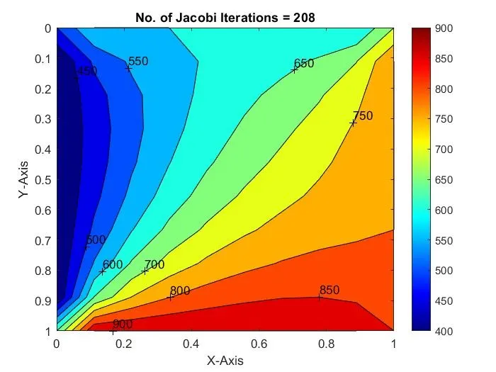
title(sprintf('No. of Jacobi Iterations = %d', jacobi_iteration));

PLOT

GAUSS SEIDEL METHOD

close all
clear all
clc

%Solving the Steady state 2D heat conduction (Gauss-seidel Method)

%Input Parameters
%Number of grid points
nx = 10;
ny = nx;

x = linspace(0,1,nx);
y = linspace(0,1,ny);

dx = x(2) - x(1);
dy = dx;

%Absolute error criteria > tolerance
err = 9e9;
tolerance = 1e-4;

%Defining Boundary conditions
T_L = 400;
T_T = 600;
T_R = 800;
T_B = 900;

T = 300*ones(nx,ny);

T(2:ny - 1, 1)  = T_L;
T(2:ny - 1, nx) = T_R;
T(1, 2:nx - 1)  = T_T;
T(ny, 2:nx - 1) = T_B;

%Calculating Average temperature at corners
T(1,1) = (T_T + T_L)/2;
T(nx,ny) = (T_R + T_B)/2;
T(1,ny) = (T_T + T_R)/2;
T(nx,1) = (T_L + T_B)/2;

%Assigning orginal values to T
T_intial = T;
T_old = T;


%Calculation of 2D steady heat conduction EQUATION by Gauss-Seidel method
iterative_solver = 2;

if iterative_solver == 2
    Gauss_seidel_iteration = 1;
    
    while(err > tolerance)
        
        for i = 2:nx - 1
            
            for j = 2:ny - 1
                T(i,j) = 0.25*(T(i-1,j) + T_old(i+1,j) + T(i,j-1) + T_old(i,j+1));
            end
            
        end
        
        err = max(max(abs(T_old - T)));
        T_old = T;
        Gauss_seidel_iteration = Gauss_seidel_iteration + 1;  
        
    end
end

%Plotting
figure(1)
contourf(x,y,T)
clabel(contourf(x,y,T))
colorbar
colormap(jet)
set(gca, 'ydir', 'reverse')

xlabel('X-Axis')
ylabel('Y-Axis')
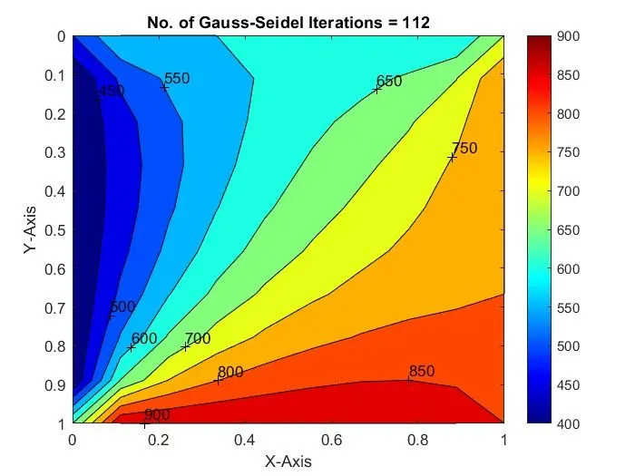
title(sprintf('No. of Gauss-Seidel Iterations = %d', Gauss_seidel_iteration));
pause(0.03);

PLOT

SOR METHOD

close all
clear all
clc

%Solving the Steady state 2D heat conduction (Successive over-relaxation Method)

%Input Parameters
%Number of grid points
nx = 10;
ny = nx;

x = linspace(0,1,nx);
y = linspace(0,1,ny);

dx = x(2) - x(1);
dy = dx;

%Absolute error criteria > tolerance
err = 9e9;
tolerance = 1e-4;
omega = 1.2;

%Defining Boundary conditions
T_L = 400;
T_T = 600;
T_R = 800;
T_B = 900;

T = 300*ones(nx,ny);

T(2:ny - 1, 1)  = T_L;
T(2:ny - 1, nx) = T_R;
T(1, 2:nx - 1)  = T_T;
T(ny, 2:nx - 1) = T_B;

%Calculating Average temperature at corners
T(1,1) = (T_T + T_L)/2;
T(nx,ny) = (T_R + T_B)/2;
T(1,ny) = (T_T + T_R)/2;
T(nx,1) = (T_L + T_B)/2;

%Assigning orginal values to T
T_intial = T;
T_old = T;


%Calculation of 2D steady heat conduction EQUATION by Successive over-relaxation method
iterative_solver = 3;

if iterative_solver == 3
    Successive_Over_Relaxation_iteration = 1;
    
    while(err > tolerance)
        
        for i = 2:nx - 1
            
            for j = 2:ny - 1
                T(i,j) = omega*(0.25*(T(i-1,j) + T_old(i+1,j) + T(i,j-1) + T_old(i,j+1))) + (1 - omega)*T_old(i,j);
            end
            
        end
        
        err = max(max(abs(T_old - T)));
        T_old = T;
        Successive_Over_Relaxation_iteration = Successive_Over_Relaxation_iteration + 1;  
        
    end
end

%Plotting
figure(1)
contourf(x,y,T)
clabel(contourf(x,y,T))
colorbar
colormap(jet)
set(gca, 'ydir', 'reverse')

xlabel('X-Axis')
ylabel('Y-Axis')
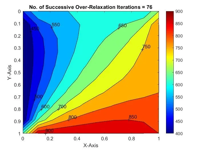
title(sprintf('No. of Successive Over-Relaxation Iterations = %d', Successive_Over_Relaxation_iteration));
pause(0.03);

PLOT

UNSTEADY STATE

CODE:

EXPLICIT

close all
clear all
clc

%Solving the Unsteady state 2D heat conduction (EXPLICIT SCHEME)

%Input Parameters
%Number of grid points
nx = 10;
ny = nx;
nt = 1400;

x = linspace(0,1,nx);
y = linspace(0,1,ny);

dx = x(2) - x(1);
dy = dx;

%Absolute error criteria > tolerance
err = 9e9;
tolerance = 1e-4;
dt = 1e-3;
omega = 1.1;

%Defining Boundary conditions
T_L = 400;
T_T = 600;
T_R = 800;
T_B = 900;

T = 300*ones(nx,ny);

T(2:ny - 1, 1)  = T_L;
T(2:ny - 1, nx) = T_R;
T(1, 2:nx - 1)  = T_T;
T(ny, 2:nx - 1) = T_B;

%Calculating Average temperature at corners
T(1,1) = (T_T + T_L)/2;
T(nx,ny) = (T_R + T_B)/2;
T(1,ny) = (T_T + T_R)/2;
T(nx,1) = (T_L + T_B)/2;

%Assigning orginal values to T
T_intial = T;
T_old = T;


%Calculation of 2D steady heat conduction EQUATION by Successive over-relaxation method
iterative_solver = 1;
k1 = 1.1*(dt/(dx^2));
k2 = 1.1*(dt/(dy^2));

if iterative_solver == 1
    Steady_Explicit = 1;
    for k = 1:nt
        err = 1; 
    
        while(err > tolerance)
        
            for i = 2:nx - 1
            
                for j = 2:ny - 1
                    Term_1 = T_old(i,j);
                    Term_2 = k1*(T_old(i+1,j) - 2*T_old(i,j) + (T_old(i-1,j)));
                    Term_3 = k2*(T_old(i,j+1) - 2*T_old(i,j) + T_old(i,j-1));
                    T(i,j) = Term_1 + Term_2 + Term_3;
                end
            
            end
        
            err = max(max(abs(T_old - T)));
            T_old = T;
            Steady_Explicit = Steady_Explicit + 1;  
        
        end
    end
end

%Plotting
figure(1)
contourf(x,y,T)
clabel(contourf(x,y,T))
colorbar
colormap(jet)
set(gca, 'ydir', 'reverse')

xlabel('X-Axis')
ylabel('Y-Axis')
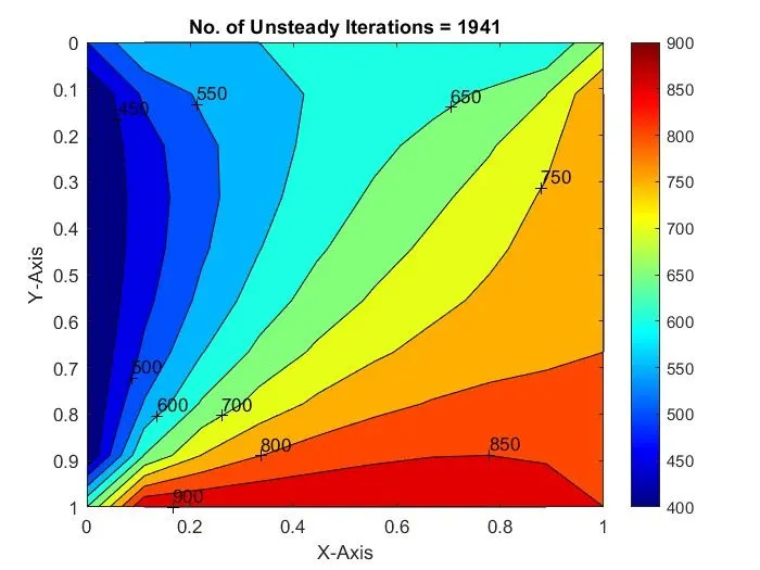
title(sprintf('No. of Unsteady Iterations = %d', Steady_Explicit));
pause(0.03);

PLOT

IMPLICIT

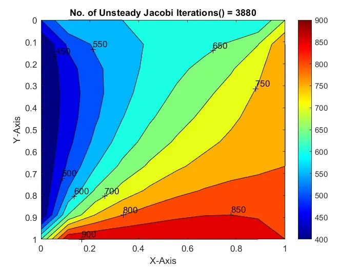
JACOBI

close all
clear all
clc

%Solving the Unsteady state 2D heat conduction by Jacobi Method(IMPLICIT SCHEME)

%Input Parameters
%Number of grid points
nx = 10;
ny = nx;
nt = 1400;

x = linspace(0,1,nx);
y = linspace(0,1,ny);

dx = x(2) - x(1);
dy = dx;

%Absolute error criteria > tolerance
error = 9e9;
tolerance = 1e-4;
dt = 1e-3;

%Defining Boundary conditions
T_L = 400;
T_T = 600;
T_R = 800;
T_B = 900;

T = 300*ones(nx,ny);

T(2:ny - 1, 1)  = T_L;
T(2:ny - 1, nx) = T_R;
T(1, 2:nx - 1)  = T_T;
T(ny, 2:nx - 1) = T_B;

%Calculating Average temperature at corners
T(1,1) = (T_T + T_L)/2;
T(nx,ny) = (T_R + T_B)/2;
T(1,ny) = (T_T + T_R)/2;
T(nx,1) = (T_L + T_B)/2;

%Assigning orginal values to T
T_old = T;
T_intial = T;

%Calculation of 2D steady heat conduction EQUATION by Successive over-relaxation method
k1 = 1.1*(dt/(dx^2));
k2 = 1.1*(dt/(dy^2));

Jacobi_iteration = 1;
for k = 1:nt
    error = 9e9; 
    
    while(error > tolerance)
        
        for i = 2:nx - 1
            
            for j = 2:ny - 1
                    
                Term_1 = 1/(1 + (2*k1) + (2*k2));
                Term_2 = k1*Term_1;
                Term_3 = k2*Term_1;
                H = (T_old(i-1,j)) + (T_old(i+1,j));
                V = (T_old(i,j+1)) + (T_old(i,j-1));
                    
                T(i,j) = (T_intial(i,j)*Term_1) + (H*Term_2) + (V*Term_3);
   
            end
            
        end
        
        error = max(max(abs(T_old - T)));
        T_old = T;
        Jacobi_iteration = Jacobi_iteration + 1;  
        
    end
    
    T_intial = T;
    
    %Plotting
    figure(1)
    contourf(x,y,T)
    clabel(contourf(x,y,T))
    colorbar
    colormap(jet)
    set(gca, 'ydir', 'reverse')

    xlabel('X-Axis')
    ylabel('Y-Axis')
    title(sprintf('No. of Unsteady Jacobi Iterations() = %d', Jacobi_iteration));
    pause(0.03)
end

PLOT

GAUSS SEIDEL

close all
clear all
clc

%Solving the Unsteady state 2D heat conduction by Gauss Seidel Method(IMPLICIT SCHEME)

%Input Parameters
%Number of grid points
nx = 10;
ny = nx;
nt = 1400;

x = linspace(0,1,nx);
y = linspace(0,1,ny);

dx = x(2) - x(1);
dy = dx;

%Absolute error criteria > tolerance
error = 9e9;
tolerance = 1e-4;
dt = 1e-3;

%Defining Boundary conditions
T_L = 400;
T_T = 600;
T_R = 800;
T_B = 900;

T = 300*ones(nx,ny);

T(2:ny - 1, 1)  = T_L;
T(2:ny - 1, nx) = T_R;
T(1, 2:nx - 1)  = T_T;
T(ny, 2:nx - 1) = T_B;

%Calculating Average temperature at corners
T(1,1) = (T_T + T_L)/2;
T(nx,ny) = (T_R + T_B)/2;
T(1,ny) = (T_T + T_R)/2;
T(nx,1) = (T_L + T_B)/2;

%Assigning orginal values to T
T_old = T;
T_intial = T;

%Calculation of 2D steady heat conduction EQUATION by Successive over-relaxation method
k1 = 1.1*(dt/(dx^2));
k2 = 1.1*(dt/(dy^2));

Gauss_Seidel_iteration = 1;
for k = 1:nt
    error = 9e9; 
    
    while(error > tolerance)
        
        for i = 2:nx - 1
            
            for j = 2:ny - 1
                    
                Term_1 = 1/(1 + (2*k1) + (2*k2));
                Term_2 = k1*Term_1;
                Term_3 = k2*Term_1;
                H = (T(i-1,j)) + (T_old(i+1,j));
                V = (T(i,j+1)) + (T_old(i,j-1));
                    
                T(i,j) = (T_intial(i,j)*Term_1) + (H*Term_2) + (V*Term_3);
   
            end
            
        end
        
        error = max(max(abs(T_old - T)));
        T_old = T;
        Gauss_Seidel_iteration = Gauss_Seidel_iteration + 1;  
        
    end
    
    T_intial = T;
    
    %Plotting
    figure(1)
    contourf(x,y,T)
    clabel(contourf(x,y,T))
    colorbar
    colormap(jet)
    set(gca, 'ydir', 'reverse')

    xlabel('X-Axis')
    ylabel('Y-Axis')
    title(sprintf('No. of Unsteady Gauss-Seidel Iterations(IMPLICIT) = %d', Gauss_Seidel_iteration));
    pause(0.03)
end

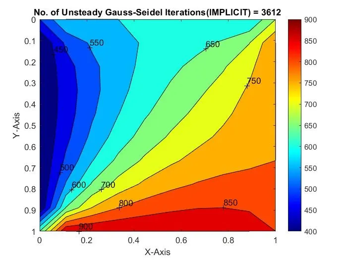
PLOT

SOR

close all
clear all
clc

%Solving the Unsteady state 2D heat conduction by Successive over-relaxation Method(IMPLICIT SCHEME)

%Input Parameters
%Number of grid points
nx = 10;
ny = nx;
nt = 1400;

x = linspace(0,1,nx);
y = linspace(0,1,ny);

dx = x(2) - x(1);
dy = dx;

%Absolute error criteria > tolerance
err = 9e9;
tolerance = 1e-4;
dt = 1e-3;
omega = 1.1;

%Defining Boundary conditions
T_L = 400;
T_T = 600;
T_R = 800;
T_B = 900;

T = 300*ones(nx,ny);

T(2:ny - 1, 1)  = T_L;
T(2:ny - 1, nx) = T_R;
T(1, 2:nx - 1)  = T_T;
T(ny, 2:nx - 1) = T_B;

%Calculating Average temperature at corners
T(1,1) = (T_T + T_L)/2;
T(nx,ny) = (T_R + T_B)/2;
T(1,ny) = (T_T + T_R)/2;
T(nx,1) = (T_L + T_B)/2;

%Assigning orginal values to T
T_old = T;
T_intial = T;
T_end = T;

%Calculation of 2D steady heat conduction EQUATION by Successive over-relaxation method
k1 = 1.1*(dt/(dx^2));
k2 = 1.1*(dt/(dy^2));

Successive_over_relaxation_iteration = 1;
for k = 1:nt
    err = 9e9; 
    
    while(err > tolerance)
        
        for i = 2:nx - 1
            
            for j = 2:ny - 1
                    
                Term_1 = 1/(1 + (2*k1) + (2*k2));
                Term_2 = k1*Term_1;
                Term_3 = k2*Term_1;
                H = (T(i-1,j)) + (T_old(i+1,j));
                V = (T(i,j+1)) + (T_old(i,j-1));
                    
                T(i,j) = (T_intial(i,j)*Term_1) + (H*Term_2) + (V*Term_3);
                T_end(i,j) = ((1-omega)*T_old(i,j)) + (T(i,j)*omega);
                
            end
            
        end
        
        err = max(max(abs(T_old - T)));
        T_old = T_end;
        Successive_over_relaxation_iteration = Successive_over_relaxation_iteration + 1;  
        
    end
    
    T_intial = T_end;
    
    %Plotting
    figure(1)
    contourf(x,y,T)
    clabel(contourf(x,y,T))
    colorbar
    colormap(jet)
    set(gca, 'ydir', 'reverse')

    xlabel('X-Axis')
    ylabel('Y-Axis')
    title(sprintf('No. of Unsteady SOR Iterations() = %d', Successive_over_relaxation_iteration));
    pause(0.03)
end

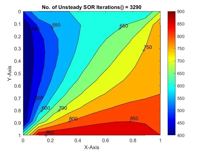
PLOT

CONCLUSION

Steady state

jacobi - 208
gasuss seidel - 112
SOR - 76

Un steady state

jacobi - 3880
gauss seidel-3612
SOR-3290
explicit - 1941

From the graphs it is clearly shown that iterations taken Jacobi>gauss>SOR for solving the steady state equation . For transient the iterative loops are more higher when compared as the time derivative functions for steady state and then converges . Most efficient is the SOR(steady state ).

Week 5.1 - Mid term project - Solving the steady and unsteady 2D heat conduction problem

Ship work like this
in your own course.

Talk to a career counsellor

Ship work like thisin your own course.

Talk to a career counsellor

Ship work like this
in your own course.