Project - Solving the steady and unsteady 2D heat conduction problem
AIM
To solve for the given 2D heat conduction with the given boundary conditions
THEORY
The 2D heat conduction equation is given by:
`(deltaT)/(delta t) - alpha ((delta^2T)/(delta x^2)+(delta^2T)/(delta y^2))=0`
`alpha`= Thermal Diffusivity. It is considered as 1.5 for our problem.
Two main approaches are used. They are steady state and transient/unsteady state. In steady state, we follow the implicit method under which three types of iterative solvers are used. They are jacobi method, gauss seidel method and successive over relaxation-method.
Under transient/unsteady state, explicit and implicit methods are used. Under implicit, again jacobi method, gauss seidel method and successive over relaxation iterative solvers are used.
One of the main differences between steady and transient states is that in steady state, the equation is time dependent. This means that CFL condition is not applicable here and the convergence is dependent on the error between consecutive iterations.
In transient state, CFL condition plays an important role in achieving convergence. Ideally the courant number should be less than 0.25 of diffusion-based equations.
The boundary conditions are given as follows:
- Top Boundary = 600 K
- Bottom Boundary = 900 K
- Left Boundary = 400 K
- Right Boundary = 800 K
The edge nodes are averaged out between their respective sides.
In steady state, the 2D heat conduction equation is:
`((delta^2T)/(delta x^2)+(delta^2T)/(delta y^2))=0` -(1)
In the implicit approach,
1. For Jacobi Method the equation becomes:
`T_P^(n+1) = (1/K)((T_L+T_R)/(Deltax^2))^n+(1/K)((T_T+T_B)/(Deltay^2))^n`
2. For Gauss Seidel Method the equation becomes:
`T_P^(n+1) = (1/K)((T_L+T_R)/(Deltax^2))^(n+1)+(1/K)((T_T+T_B)/(Deltay^2))^(n+1)`
3. For Successive Over-Relaxation Method the equation becomes:
`T_P^(n+1) = (1-omega)*T_P^(n)+omega*((1/K)((T_L+T_R)/(Deltax^2))^(n+1)+(1/K)((T_T+T_B)/(Deltay^2))^(n+1))`
Where,
TP = Temperature at present node. [T(i,j)]
TL= Temperature at the node which is on the left of present node.
TR = Temperature at the node which is on the right of present node.
TT= Temperature at the node which is on the top of present node.
TB= Temperature at the node which is on the bottom of present node.
K=`(2*(Deltax^2+Deltay^2))/(Deltax^2*Deltay^2)`
`omega`=relaxation factor. It is take as 1.2.
In transient state, the 2D heat conduction equation is:
`(deltaT)/(delta t) = alpha ((delta^2T)/(delta x^2)+(delta^2T)/(delta y^2))`
In the explicit approach,
The equation is:
`T_P^(n+1) = T_P^n + k1*(T_L-2T_P+T_R)^n+ k2*(T_T-2T_P+T_B)^n`
Where,
TP = Temperature at present node. [T(i,j)]
TL= Temperature at the node which is on the left of present node.
TR = Temperature at the node which is on the right of present node.
TT= Temperature at the node which is on the top of present node.
TB= Temperature at the node which is on the bottom of present node.
k1 = `alpha*(Deltat)/(Deltax^2)`
k2 = `alpha*(Deltat)/(Deltay^2)`
k1 and k2 are CFL conditions who should be less than 0.25.
In the implicit approach,
1. For Jacobi Method the equation becomes:
`T_P^(n+1) = (1/(1+2k1+2k2))*[T_P^n+k1(T_L+T_R)^n+k2(T_T+T_B)^n]`
2. For Gauss Seidel Method the equation becomes:
`T_P^(n+1) = (1/(1+2k1+2k2))*[T_P^n+k1(T_L^(n+1)+T_R^n)+k2(T_T^n+T_B^(n+1))]`
3. For Successive Over-Relaxation Method the equation becomes:
`T_P^(n+1) = (1-omega)*T_P^n+[omega*(1/(1+2k1+2k2))*[T_P^n+k1(T_L^(n+1)+T_R^n)+k2(T_T^n+T_B^(n+1))]]`
CODE
1. STEADY STATE IMPILICT METHOD
clear all
close all
clc

%nodes on x and y direction
nx = 10;
ny = 10;
%error tolerance
tolerance = 1e-4;
%initializiing error
error = 10;
%mesh
x=linspace(0,1,nx);
y=linspace(0,1,ny);

dx = x(2)-x(1);
dy = y(2)-y(1);

%meshgrid to obtain 2d matrix
[X Y]=meshgrid(x,y);

%defining k
k = ((2*((dx^2)+(dy^2)))/((dx^2)*(dy^2)));

%omega value for SOR method
omega=1.2;

%initial conditions (BCs)
t=300*ones(nx,ny);
t(1,:)=600;%top
t(end,:)=900;%bottom
t(:,1)=400;%left
t(:,end)=800;%right
%edges of intitial conditions(BCs)
t(1,1)=((t(1,2)+t(2,1))/2);
t(1,end)=((t(1,end-1)+t(2,end))/2);
t(end,end)=((t(end-1,end)+t(end,end-1))/2);
t(end,1)=((t(end-1,1)+t(end,2))/2);
%making copies of t for later use
t_old=t;
t_initial=t;
iterative_solver = 1;
% loops for iterative solvers

%jacobi method
if iterative_solver == 1%convergence loop
    jacobi_iter=1; %initialize iter counter
    while (error > tolerance)%error loop
        for i=2:(nx-1)%space loop
            for j=2:(ny-1)
                term1=((t_old(i-1,j)+t_old(i+1,j))/(dx^2));
                term2=((t_old(i,j+1)+t_old(i,j-1))/(dy^2));
                t(i,j)=(term1+term2)/k;
            end
        end
        error=max(max(abs(t_old-t)));%error update
        t_old=t;%update t_old with new iter values;
        jacobi_iter=jacobi_iter+1;%update iter counter
        [m,n]=contourf(X,Y,t,'--');%contour plot
        set(gca,'ydir','reverse')
        colorbar
        colormap(turbo)
        clabel(m,n)
        title_text = sprintf('Steady State Implicit - Jacobi Method. n Total no. of interations = %d',jacobi_iter);
        title(title_text)
        pause(0.03)

    end
end

%GS method
if iterative_solver == 2%convergence loop
    gs_iter=1; %initialize iter counter
    while (error > tolerance)%error loop
        for i=2:(nx-1)%space loop
            for j=2:(ny-1)
                term1=((t(i-1,j)+t_old(i+1,j))/(dx^2));
                term2=((t_old(i,j+1)+t(i,j-1))/(dy^2));
                t(i,j)=(term1+term2)/k;
            end
        end
        error=max(max(abs(t_old-t)));%error update
        t_old=t;%update t_old with new iter values;
        gs_iter=gs_iter+1;%update iter counter
        [m,n]=contourf(X,Y,t,'--');%contour plot
        set(gca,'ydir','reverse')
        colorbar
        colormap(turbo)
        clabel(m,n)
        title_text = sprintf('Steady State Implicit - Gauss Seidel Method. n Total no. of interations = %d',gs_iter);
        title(title_text)
        pause(0.03)

    end
end

%SOR method
if iterative_solver == 3%convergence loop
    sor_iter=1; %initialize iter counter
    while (error > tolerance)%error loop
        for i=2:(nx-1)%space loop
            for j=2:(ny-1)
                term1=((t(i-1,j)+t_old(i+1,j))/(dx^2));
                term2=((t_old(i,j+1)+t(i,j-1))/(dy^2));
                term=(term1+term2)/k;
                t(i,j)=((1-omega)*t_old(i,j))+(omega*term);
            end
        end
        error=max(max(abs(t_old-t)));%error update
        t_old=t;%update t_old with new iter values;
        sor_iter=sor_iter+1;%update iter counter
        [m,n]=contourf(X,Y,t,'--');%contour plot
        set(gca,'ydir','reverse')
        colorbar
        colormap(turbo)
        clabel(m,n)
        title_text = sprintf('Steady State Implicit - SOR Method. n Total no. of interations = %d',sor_iter);
        title(title_text)
        pause(0.03)

    end
end
2. TRANSIENT STATE CODES
2.1 EXPLICIT FUNCTION CODE
function [explicit_time,error]=transient_explicit(t,t_old,k1,k2,nt,nx,ny,tolerance,X,Y)
    explicit_iter=1;
    tic
    for q=1:nt  %time loop
        error =9e9;
        while (error>tolerance) %error loop
            for i=2:nx-1    %spatial loop
                for j=2:ny-1    %spatial loop
                    term1=(t_old(i-1,j)-(2*t_old(i,j))+t_old(i+1,j));
                    term2=(t_old(i,j-1)-(2*t_old(i,j))+t_old(i,j+1));
                    t(i,j)=t_old(i,j)+(k1*term1)+(k2*term2);
                end
            end
            error=max(max(abs(t_old-t)));   %error update
            t_old=t;    %update t_old with new iter values;
            explicit_iter=explicit_iter+1;  %update iter counter
        end
    end
    explicit_time=toc   %store computation time
    figure(1)
    [m,n]=contourf(X,Y,t,'--'); %contour plot
    set(gca,'ydir','reverse') %reversing y axis
    colorbar
    colormap(turbo)
    clabel(m,n)
    title_text = sprintf('Transient State - Explicit Method. n Total No. Of Iterations =  %d',explicit_iter);
    title(title_text)
end
2.2 IMPLICIT JACOBI FUNCTION CODE
function [time_imp_jacobi,error]=transient_implicit_jacobi(t,t_old,k1,k2,nt,nx,ny,tolerance,t_pre,X,Y)
        jacobi_iter=1;
        tic
        for q=1:nt  %time loop
            error =9e9;
            while(error>tolerance) %error loop
                for i=2:nx-1    %spatial loop
                    for j=2:ny-1    %spatial loop
                        k=(1/(1+(2*k1)+(2*k2)));
                        term1=t_old(i-1,j)+t_old(i+1,j);
                        term2=t_old(i,j-1)+t_old(i,j+1);
                        t(i,j) = k*(t_pre(i,j)+(k1*term1)+(k2*term2));
                    end
                end
                error = max(max(abs(t_old-t)));
                t_old=t;
                jacobi_iter=jacobi_iter+1;
            end
            t_pre=t;
        end
        time_imp_jacobi=toc %store computation time
        figure(2)
        [m,n]=contourf(X,Y,t,'--'); %contour plot
        set(gca,'ydir','reverse')%reversing y axis
        colorbar
        colormap(turbo)
        clabel(m,n)
        title_text = sprintf('Transient State - Implicit - Jacobi Method. n Total No. Of Iterations = %d',jacobi_iter);
        title(title_text)
end
2.3 IMPLICIT GAUSS SEIDEL FUNCTION CODE
function [time_imp_gauss,error]=transient_implicit_gauss(t,t_old,k1,k2,nt,nx,ny,tolerance,t_pre)
        gauss_iter=1;
        tic
        for q=1:nt  %time loop
            error =9e9;
            while(error>tolerance)  %error loop
                for i=2:nx-1    %spatial loop
                    for j=2:ny-1    %spatial loop
                        k=(1/(1+(2*k1)+(2*k2)));
                        term1=t(i-1,j)+t_old(i+1,j);
                        term2=t(i,j-1)+t_old(i,j+1);
                        t(i,j) = k*(t_pre(i,j)+(k1*term1)+(k2*term2));
                    end
                end
                error = max(max(abs(t_old-t)));%calculate error
                t_old=t;%update t_old
                gauss_iter=gauss_iter+1;%update iter no.
            end
            t_pre=t;  %update prev value of t
        end
        time_imp_gauss=toc%store computation time
        figure(3)
        [m,n]=contourf(t,'--'); %contour plot
        set(gca,'ydir','reverse') %reversing y axis
        colorbar
        colormap(turbo)
        clabel(m,n)
        title_text = sprintf('Transient State - Implicit - Gauss Seidel Method. n Total no of Iterations = %d',gauss_iter);
        title(title_text)
end
2.4 IMPLICIT SOR FUNCTION CODE
function [time_imp_sor,error]=transient_implicit_sor(t,t_old,k1,k2,nt,nx,ny,tolerance,t_pre,omega)
        sor_iter=1;
        tic
        for q=1:nt  %time loop
            error =9e9;
            while(error>tolerance) %error loop
                for i=2:nx-1    %spatial loop
                    for j=2:ny-1    %spatial loop
                        k=(1/(1+(2*k1)+(2*k2)));
                        term1=t(i-1,j)+t_old(i+1,j);
                        term2=t(i,j-1)+t_old(i,j+1);
                        t(i,j) =((1-omega)*t_old(i,j)) + (omega*(k*(t_pre(i,j)+(k1*term1)+(k2*term2))));
                    end
                end
                error = max(max(abs(t_old-t)));%calculate error
                t_old=t;%update t_old
                sor_iter=sor_iter+1;%update iter no.
            end
            t_pre=t;  %update prev value of t
        end
        time_imp_sor=toc    %store computation time
        figure(4)
        [m,n]=contourf(t,'--'); %contour plot
        set(gca,'ydir','reverse') %reversing y axis
        colorbar
        colormap(turbo)
        clabel(m,n)
        title_text = sprintf('Transient State - Implicit - SOR Method. n Total No. Of Iterations = %d',sor_iter);
        title(title_text)
end
2.5 MAIN CODE
clear all
close all
clc


%nodes on x and y direction
nx = 10;
ny = 10;
%error tolerance
tolerance = 1e-4;
%initializiing error
error = 10;
%mesh
x=linspace(0,1,nx);
y=linspace(0,1,ny);

dx = x(2)-x(1);
dy = y(2)-y(1);

%meshgrid to obtain 2d matrix
[X Y]=meshgrid(x,y);

%alpha and omega values
alpha = 1.5;    %thermal diffusivity
omega=1.2;  %relaxation factor
time = 5;
dt=0.001;   %from cfl hand calc
nt=time/dt;

%defining k1 and k2
k1 = alpha*(dt/(dx^2));
k2 = alpha*(dt/(dy^2));

%initial conditions (BCs)
t=300*ones(nx,ny);
t(1,:)=600; %top
t(end,:)=900;   %bottom
t(:,1)=400; %left
t(:,end)=800;   %right

%edges of intitial conditions(BCs)
t(1,1)=((t(1,2)+t(2,1))/2);
t(1,end)=((t(1,end-1)+t(2,end))/2);
t(end,end)=((t(end-1,end)+t(end,end-1))/2);
t(end,1)=((t(end-1,1)+t(end,2))/2);

%making copies of t for later use
t_old=t;
t_pre=t;

%calling functions to find explicit and implicit solutions
[time_explicit,error_explicit]=transient_explicit(t,t_old,k1,k2,nt,nx,ny,tolerance,X,Y);

[time_imp_jacobi,error_imp_jacobi]=transient_implicit_jacobi(t,t_old,k1,k2,nt,nx,ny,tolerance,t_pre,X,Y);

[time_imp_gauss,error_imp_gauss]=transient_implicit_gauss(t,t_old,k1,k2,nt,nx,ny,tolerance,t_pre);

[time_imp_sor,error_imp_sor]=transient_implicit_sor(t,t_old,k1,k2,nt,nx,ny,tolerance,t_pre,omega);
CODE EXPLAINATION
1. STEADY STATE
- First, variables are created for all known values and stored. Also, constants which will be used later are also created.
- Using nested loops, the iterative methods are coded.
- An if-elseif condition selects the iterative method. Then a while loop ensures that the required error’s tolerance value is achieved. Inside the while loop, for loops are used to find the temperature values based on the equations mentioned above in the theory.
- The while (error) loop runs until error value is less than 1e-4.
- It is important to ensure old values are updated outside the error loop after finding the error value. Contour plots are created with suitable colormap and title. The y axis direction is reversed to get the desired output.
2. TRANSIENT STATE
- In transient state, the code complexity increases. So, functions are created for explicit, implicit-jacobi, gauss seidel and SOR methods.
- These functions take values from the main code which are created based on the assumptions, boundary conditions and the CFL condition.
- The CFL number should be less than 0.25. So, dt is taken as 0.001, which gives an approximate CFL number of 0.12. This also results in the number of timesteps (shown as nt in code) to be 5000.
- Each functions’ structures are similar. They all contain a time loop which has an error loop in it. The error loop has the spatial loop in it.
- The plot is plotted using contourf command. The y axis direction is reversed to get the desired output. The plot code is outside all loops to aid faster computation time.
- The error loop runs until error value is less than 1e-4.
- It is important to ensure old values are updated outside the spatial loop to obtain desired results.
- Iteration counters are also created for later use in comparisons.
RESULTS
1. Steady State
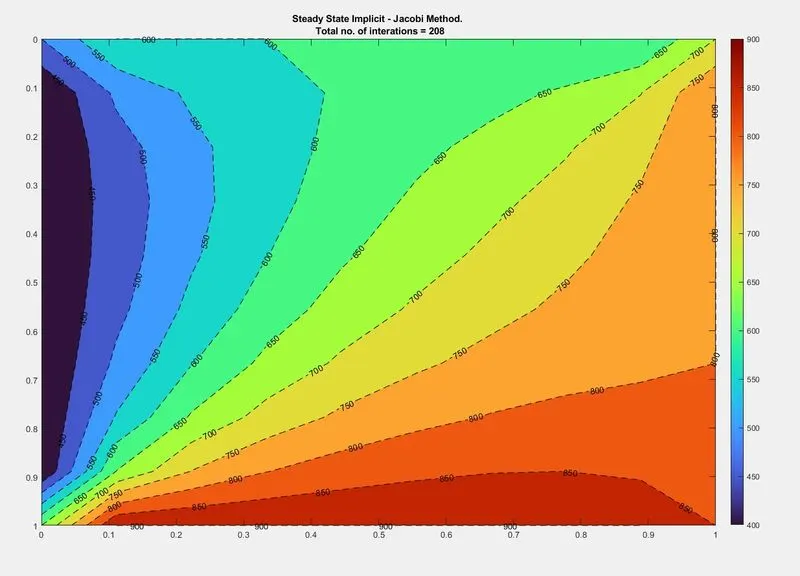
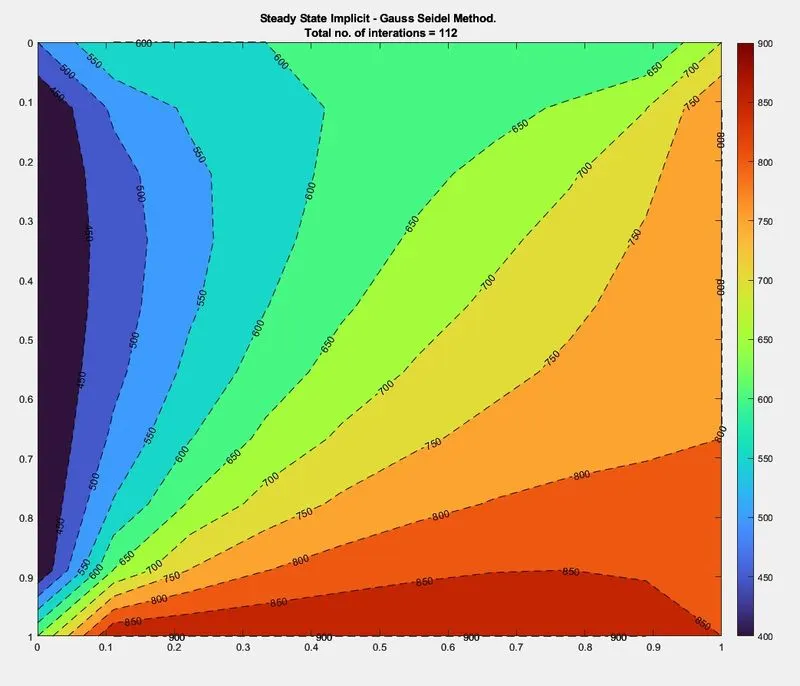
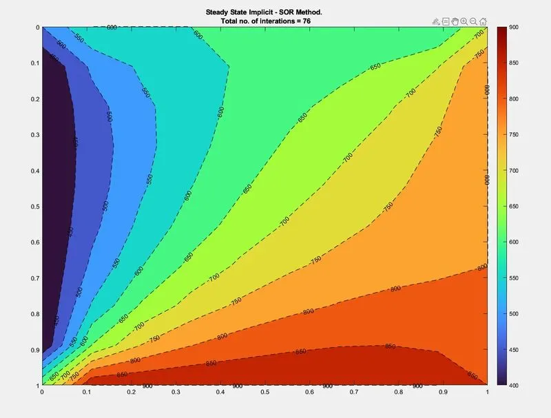
In all 3 methods, the solution converges but the number of iterations vary. Successive over-relxation take the least number of iterations at 76 iterations. Then , gauss-seidel method takes 112 iterations. Jacobi method has the hight iterations of all three methods at 208 iterations.
2. Transient State
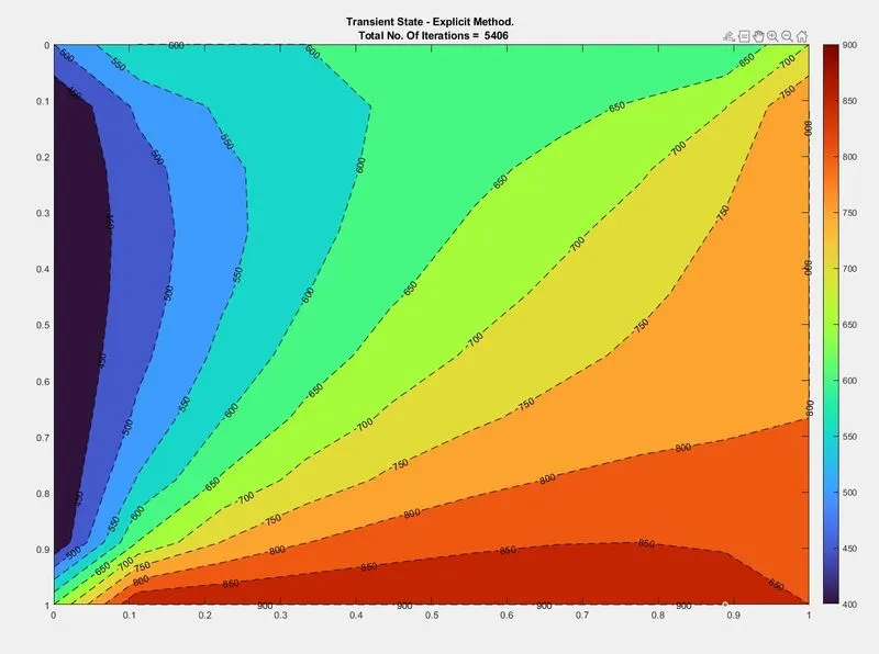
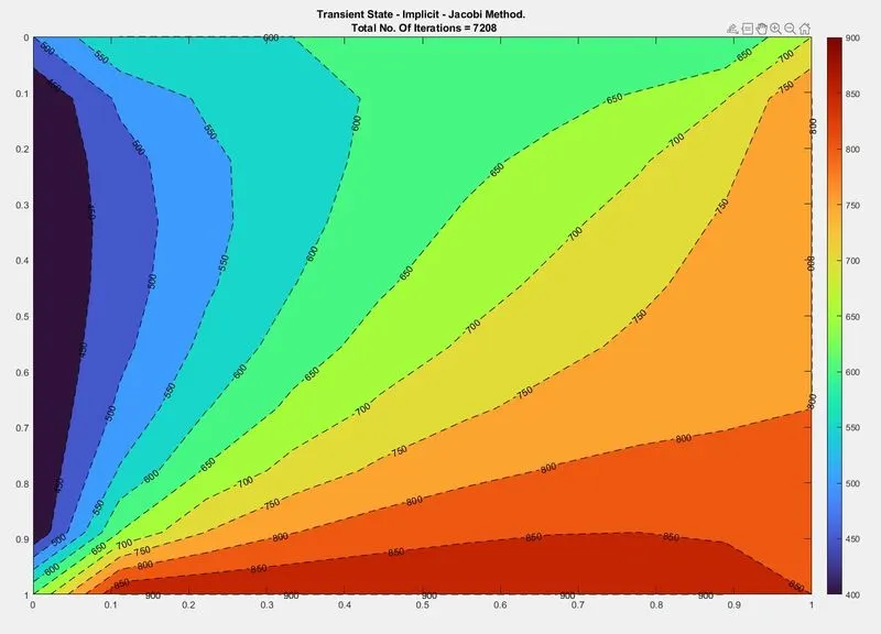
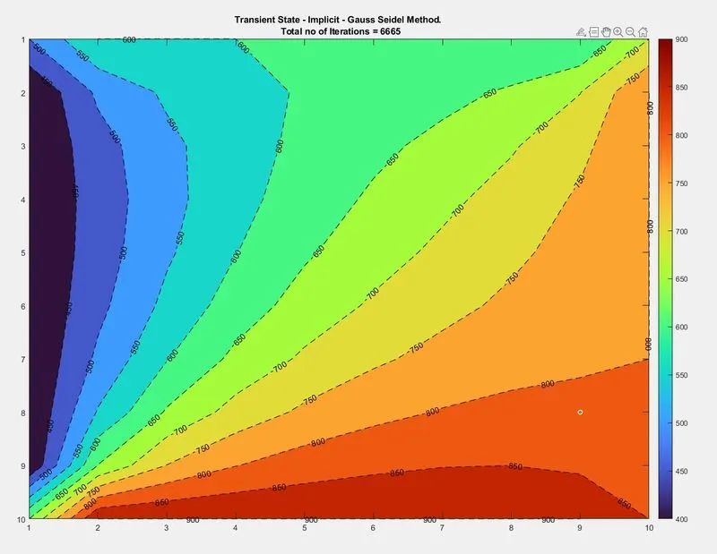
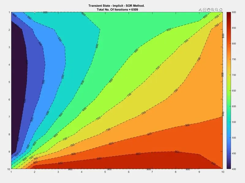
- The explicit approach in transient state takes a total of 5406 iterations.
- In the implicit approach, like the steady state implicit results, successive over-relaxation method has the lowest iterations and the jacobi method the highest.
- Successive over-relaxation method takes 6509 iterations.
- Gauss Seidel method takes 6665 iterations.
- Jacobi method takes 7208.