Week 5.1 - Mid term project - Solving the steady and unsteady 2D heat conduction problem
-
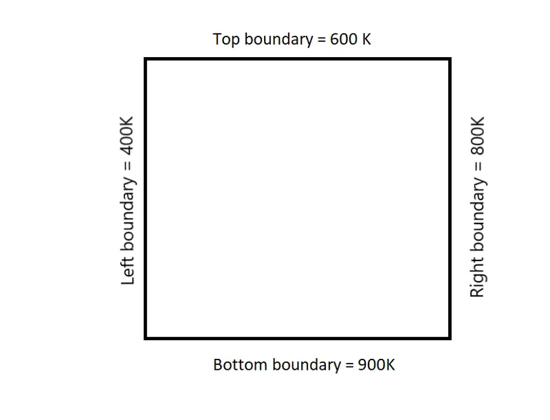
Solve the 2D heat conduction equation by using the point iterative techniques that were taught in the class. The Boundary conditions for the problem are as follows;
Top Boundary = 600 K
Bottom Boundary = 900 K
Left Boundary = 400 K
Right Boundary = 800 K
-
The following methods for solving implicit equations.
1. Jacobi
2. Gauss-seidel
3. Successive over-relaxation
- Objective - To write a code for 2D heat conduction equation by using iterative techniques.The methods to solve the implicit equations are jacobi, gauss-seidel, successive over-relaxation.Then the Implicit and Explicit method is also considered. Finally, the most efficient method for solving 2D heat conduction in the steady and transient case is concluded by taking both the number of iterations and the time required to solve the simulation.
- The accuracy of the solution obtained by the explicit and implicit method should be in accordance with the specified tolerance value.
- Write code for both implicit and explicit schemes.
- In transient analysis ,equations can be solved either in implicit form or in its explicit form.
-
2D heat conduction equation is
(∂T /∂t)+α⋅(∂^2T /∂x^2+∂^2T /∂y^2)=0
T is temperature and t is time.
For steady-state Time derivative will be zero hence the equation will be;
α⋅(∂^2T /∂x^2+∂^2T / ∂y^2)=0
- Heat conduction in the medium is generally three-dimensional and time-dependent, and the temperature in the medium varies with position and time, i.e.is, T(x, y, z, t). Conduction of heat in a medium is said to be stable when
the temperature does not change with time and is unstable or transient.-
For an unsteady state the 2-D heat conduction equation is represented as :
∂T∂t=α⋅(∂2T∂x2+∂2T∂y2)">∂T /∂t=α⋅(∂^2T /∂x^2+∂^2T /∂y^2)
For a steady state condition, the heat conduction equation is represented as :
(∂2T∂x2+∂2T∂y2)=0">(∂^2T /∂x^2+∂^2T /∂y^2)=0
-
- The boundary conditions for the problem are as given below :
- Jacobi method - Jacobi's method, or Jacobi's method, is one of the iterative methods for approximating the solution of a system of n linear equations in n variables.
- The Jacobi iteration method is considered an iterative algorithm that is used to determine the solution of a system of linear equations in numerical linear algebra that is diagonally dominant. This method fills in an approximate value for each diagonal element.
- Gauss-seidel method-In numerical linear algebra, the Gauss–Seidel method, also known as the Liebmann method or the stepwise displacement method, is an iterative method used to solve a system of linear equations. The Gauss-Seidel method is an iterative technique for solving a quadratic system of n linear equations with unknown x.
- Successive over-relaxation method- In numerical linear algebra, the method of successive over-relaxation (SOR) is a variant of the Gauss-Seidel method for solving a linear system of equations, resulting in faster convergence. A similar method can be used for any slowly converging iterative process.
- Transient Analysis using the explicit scheme
-
clear all close all clc %Input parameters nx =10 ny =10 nx =ny dt = 0.001 alpha = 1.4 nt = 200 T = ones(nx ,ny) %initial conditions for i = 1:nx T(1,i) = 600; T(nx,i)= 900 ; end for j=1:ny T(j,1) = 400 ; T(j,ny)= 800 ; end T(1,1)= (T(1,2)+ T(2,1))/2; T(1,nx) = (T(1,nx-1)+T(2,nx))/2; T(ny,1) = (T(ny-1,1) + T(ny,2))/2; T(ny,nx) = (T(ny,nx-1)+T(ny-1,nx))/2; %Creating array x =linspace(0 ,1,nx) y =linspace(0 ,1,ny) dx = x(2) -x(1) dy = y(2)-y(1) Told = T %CFL values for stablity k1 = alpha*(dt/dx^2) k2 = alpha*(dt/dy^2) %Time loop for k=1:nt for i =2:nx-1 for j= 2:ny-1 T(i,j) = (Told(i,j) + (k1*(Told(i+1,j)-(2*Told(i,j))+Told(i-1,j))) + (k2*(Told(i,j-1)-(2*Told(i,j)) +Told(i,j+1)))); end end Told = T %plotting figure(1) colormap(jet) A=contourf(x,y,T); clabel(A); set(gca,'YDir','reverse'); colorbar; xlabel('x direction') ylabel('y direction') grid on ; title (' Transient Analysis of 2D-heat conduction equation using explicit scheme'); B = sprintf(' Number of timesteps = %d, timestep (dt) = %d',k,dt); subtitle(B); pause(0.0001); end - Stepwise Explaination of the code-
- Code started with clear ,close ,clc command.
%Input parameters are given ,
- Boundary conditions are given to execute the for loop:
-
Top Boundary = 600 K
Bottom Boundary = 900 K
Left Boundary = 400 K
Right Boundary = 800 K
- For loop is used to store the values .
- Boundary conditions are stored in case of temperature for no.of nodes in x direction and no. of nodes in y ditrection.
- Then linspace command is used to execute the array function.
- CFL formula is used to calculate the CFL values for stability.
- Time loop command is given and for loop is used to execute timesteps.
- x-direction vs y-direction graph are plotted.
- Results-
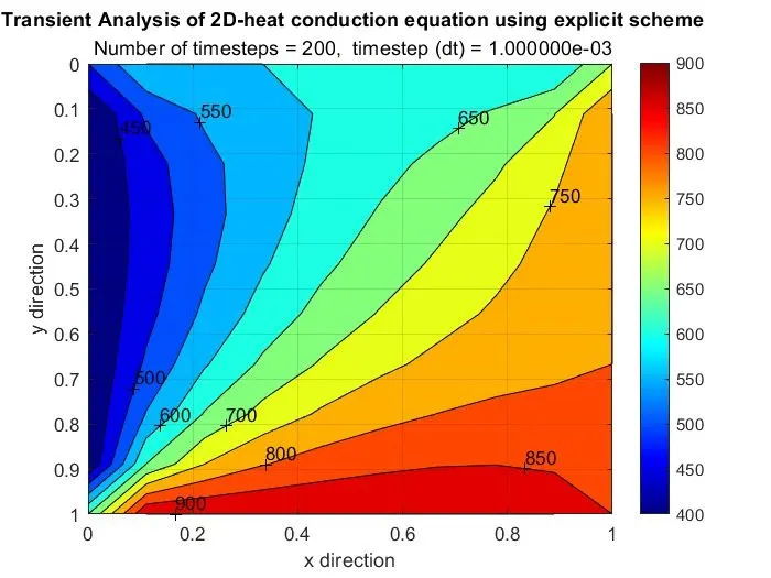
- The graph is programmed in a time loop to record changes in the temperature distribution at each time step.
- The solution reaches a steady state before the specified number of time steps. If the time step size (dt) varies accordingly, the time required to reach steady state will also vary.
- For the current timestep of 0.001 the solution reaches a steady state at around 100 to 150 iterations.
- Node size and thermal diffusivity also affecting the steady state solution.
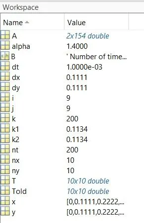
- CFL is directly proportional to dt ,so as decreasing the temperature CFL also decreases.
- CFL should be less than or equal to 0.5.
- Transient Analysis using the implicit scheme-
- The three iterative methods indicated above are used in the following MATLAB program.
clear all
close all
clc
%Input parameters
nx =10
ny =10
nx =ny
dt = 0.002
alpha = 1.4
nt = 200

T = ones(nx ,ny)
%initial conditions
for i = 1:nx
    T(1,i) = 600;
    T(nx,i)= 900 ;
end
for j=1:ny
    T(j,1) = 400 ;
    T(j,ny)= 800 ;
end

T(1,1)= (T(1,2)+ T(2,1))/2;
T(1,nx) = (T(1,nx-1)+T(2,nx))/2;
T(ny,1) = (T(ny-1,1) + T(ny,2))/2;
T(ny,nx) = (T(ny,nx-1)+T(ny-1,nx))/2;

%Creating array
x =linspace(0 ,1,nx)
y =linspace(0 ,1,ny)

dx = x(2) -x(1)
dy = y(2)-y(1)

Told = T

iteration = 3
tol = 1e-4

%CFL values for stablity
k1 = alpha*(dt/dx^2)
k2 = alpha*(dt/dy^2)

Tprev = T
iter = 1

%Jacobi method
if iteration==1

%Time loop
for k =1:1200

 error = 9e9

 %Convergence loop
 while(error>tol)

   for i =2:nx-1
   for j= 2:ny-1

 term1 = (1/(1+(2*k1)+(2*k2)));
  term2 = k1*term1;
  term3 = k2*term1;
  T(i,j) = (term1*Tprev(i,j)) + (term2*(Told(i+1,j)+Told(i-1,j))) + (term3*(Told(i,j-1)+Told(i,j+1)));

   end
   end

   %Calculating maximum error value
   error = max(max(abs(Told-T)))
   Told = T
   iter = iter + 1

 end
 Tprev = T
end
end

%Gauss-siedel method
if iteration==2

%Time loop
for k =1:1200

 error = 9e9

 %Convergence loop
 while(error>tol)

   for i =2:nx-1
   for j= 2:ny-1

 term1 = (1/(1+(2*k1)+(2*k2)));
  term2 = k1*term1;
  term3 = k2*term1;
  T(i,j) = (term1*Tprev(i,j)) + (term2*(Told(i+1,j)+T(i-1,j))) + (term3*(T(i,j-1)+Told(i,j+1)));

   end
   end

   %Calculating maximum error value
   error = max(max(abs(Told-T)))
   Told = T
   iter = iter + 1

 end
 Tprev = T
end
end

%SOR Method
if iteration==3
   omega = 1.013;

%Time loop
for k =1:1200

 error = 9e9

 %Convergence loop
 while(error>tol)

   for i =2:nx-1
   for j= 2:ny-1

 term1 = (1/(1+(2*k1)+(2*k2)));
  term2 = k1*term1;
  term3 = k2*term1;
   T(i,j) = ((1-omega)*Told(i,j)) + omega*((term1*Tprev(i,j)) + (term2*(Told(i+1,j)+T(i-1,j))) + (term3*(T(i,j-1)+Told(i,j+1))));
   end
   end

   %Calculating maximum error value
   error = max(max(abs(Told-T)))
   Told = T
   iter = iter + 1

 end
 Tprev = T
end
end
%plotting
figure(1)
colormap(jet)
A=contourf(x,y,T);
clabel(A);
set(gca,'YDir','reverse');
colorbar;
xlabel('x direction')
ylabel('y direction')
grid on ;
title (' Transient Analysis of 2D-heat conduction equation using implicit scheme');
B = sprintf(' Number of timesteps = %d,  timestep (dt) = %d',k,dt);
subtitle(B);
pause(0.0001);
- In this code three iterative solvers are used.
- Iteration =1 ,this solver uses the jacobi method.
- Iteration =2, this solver uses the Gauss-siedel method.
- Iteration=3,this solver uses the successive over relaxation method.
- Results- Jacobi method
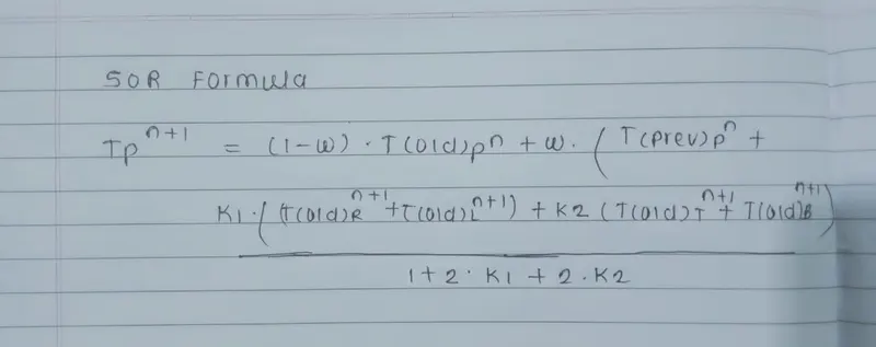
- Formula-
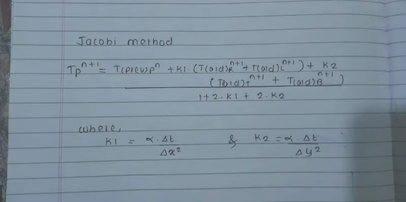
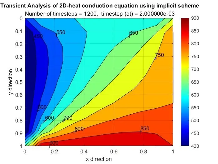
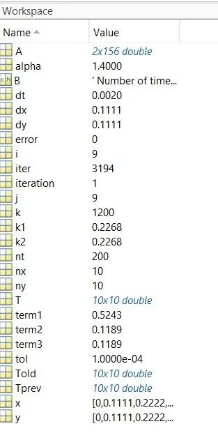
- Gauss-Siedel method -formula
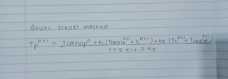
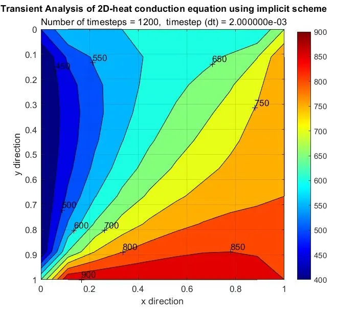
Iteration = 2 , Iter = 2607 , Number of timsteps = 1200
- successive over relaxation method.
- Formula
-
- Steady state analysis of 2D heat conduction problem
For a steady state condition, the heat conduction equation is represented as :
(∂^2T /∂x^2+∂^2T /∂y^2)=0
- In this code three iterative solvers are used.
- Iteration =1 ,this solver uses the jacobi method.
- Iteration =2, this solver uses the Gauss-siedel method.
- Iteration=3,this solver uses the successive over relaxation method.
clear all
close all
clc

%Input parameters
nx =10
ny =10
nx =ny
dt = 0.003
alpha = 1.4

 T = ones(nx ,ny)

%initial conditions
for i = 1:nx
    T(1,i) = 600;
    T(nx,i)= 900 ;
end
for j=1:ny
    T(j,1) = 400 ;
    T(j,ny)= 800 ;
end

T(1,1)= (T(1,2)+ T(2,1))/2;
T(1,nx) = (T(1,nx-1)+T(2,nx))/2;
T(ny,1) = (T(ny-1,1) + T(ny,2))/2;
T(ny,nx) = (T(ny,nx-1)+T(ny-1,nx))/2;

%Creating array
x =linspace(0 ,1,nx)
y =linspace(0 ,1,ny)

dx = x(2) -x(1)
dy = y(2)-y(1)

Told = T

%CFL values for stablity
k1 = alpha*(dt/dx^2)
k2 = alpha*(dt/dy^2)

%Selection of the iterative solver method
iteration =1

% tolerance
tol = 1e-4;
error = 1e4;

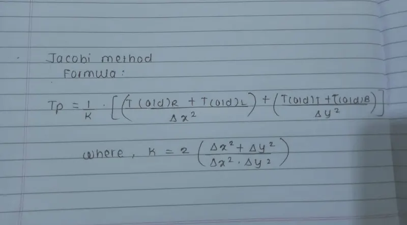
k = ((2*(dy^2 + dx^2))/(dy^2*dx^2));

%Jacobi method
if iteration==1
    iter =1

while(error>tol)

   for i =2:nx-1
   for j= 2:ny-1

    term_1 = ((Told(i+1,j) + Told(i-1,j))/(k*dx^2));
    term_2 = ((Told(i,j-1) + Told(i,j+1))/(k*dy^2));
    T(i,j) = term_1 + term_2;

end
   end

   %Calculating maximum error value
   error = max(max(abs(Told-T)))
   Told = T
   iter = iter + 1

    end
 Tprev = T
end

%Gauss-siedel method
if iteration==2
  iter =1

while(error>tol)

   for i =2:nx-1
   for j= 2:ny-1

    term_1 = ((Told(i+1,j) + Told(i-1,j))/(k*dx^2));
    term_2 = ((Told(i,j-1) + Told(i,j+1))/(k*dy^2));
    T(i,j) = term_1 + term_2;

end
   end

   %Calculating maximum error value
   error = max(max(abs(Told-T)))
   Told = T
   iter = iter + 1

    end
 Tprev = T
end

%SOR Method
if iteration==3
   omega = 1.013;

iter =1

while(error>tol)

   for i =2:nx-1
   for j= 2:ny-1

   term_1 = ((Told(i+1,j) + T(i-1,j))/(k*dx^2));
   term_2 = ((T(i,j-1) + Told(i,j+1))/(k*dy^2));
   T(i,j) = ((Told(i,j)*(1-omega)) + omega*(term_1 + term_2));

  end
   end

   %Calculating maximum error value
   error = max(max(abs(Told-T)))
   Told = T
   iter = iter + 1

    end
 Tprev = T
end
%plotting
figure(1)
colormap(jet)
A=contourf(x,y,T);
clabel(A);
set(gca,'YDir','reverse');
colorbar;
xlabel('x direction')
ylabel('y direction')
grid on ;
title (' Steady State Analysis of 2D-heat Conduction equation ');
B = sprintf(' Number of timesteps = %d,  timestep (dt) = %d',k,dt);
subtitle(B);
pause(0.0001);
- Results-
- Jacobi formula-
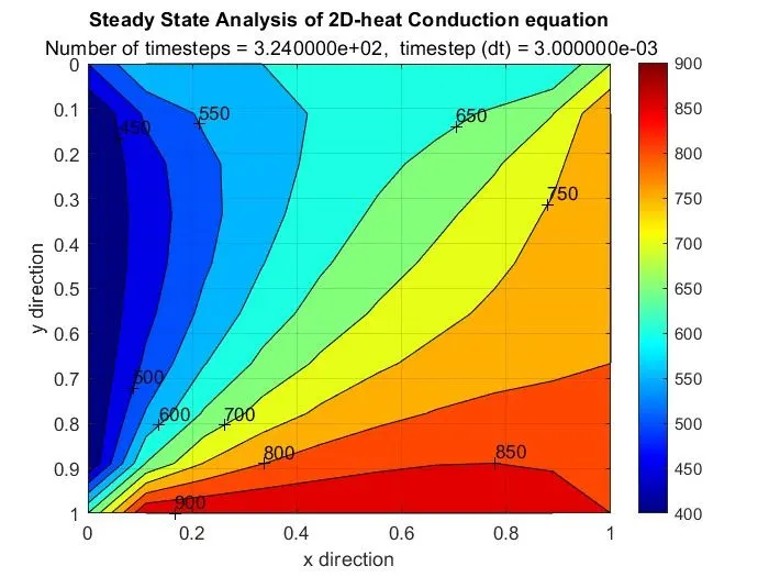
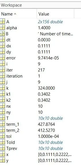
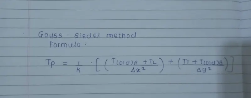
- Gauss siedel method
- Formula
-
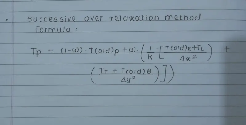
- SOR METHOD
- formula
-
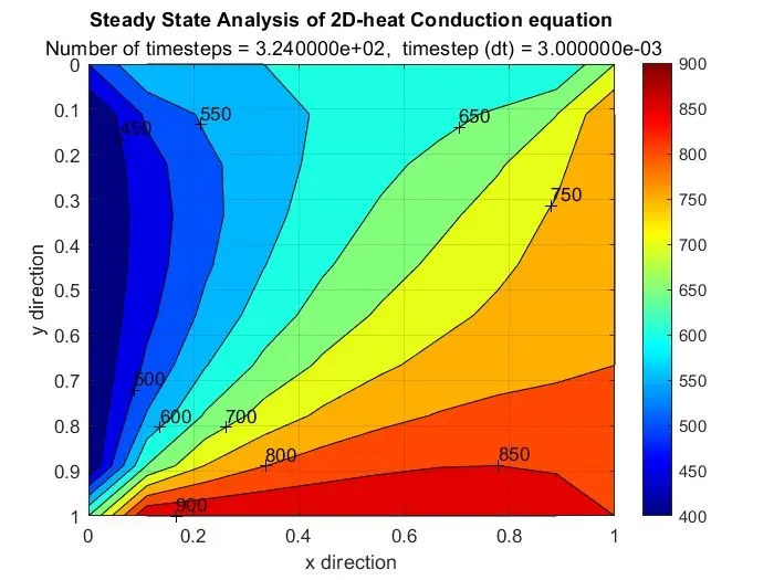
Conclusion- The maximum number of iterations can be seen with the jacobi method. So the trend in terms of number of iterations for convergence is :
Jacobi method > Gauss-siedel method > SOR method.