Week 5.1 - Mid term project - Solving the steady and unsteady 2D heat conduction problem
Objective:
To solve the 2D heat conduction problem for the steady and unsteady state using Jacobi, gauss seidel, and successive over-relaxation iterative techniques.
Theory:
Conduction is a way that heat moves from one place to another. It usually happens in solids because of differences in temperature caused by free electrons and lattice vibration.
A general equation for conduction is given.
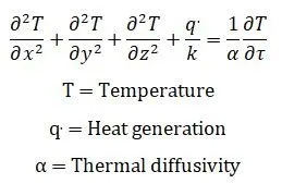
Thermal diffusivity is a thermophysical property of a material that is defined as the ratio of the material's thermal conductivity to its thermal capacity.
Since the problem is only in two dimensions and there is no heat generation, these terms are not taken into account. So, the equation shows the unsteady heat flow in two dimensions (parabolic).
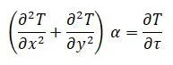
For steady-state, the time derivative is not taken into account. The 2D steady-state heat conduction equation is shown below (elliptic).
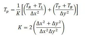
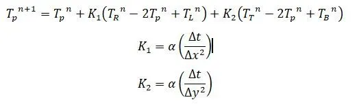
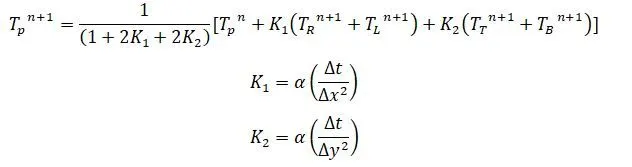
Here iterative methods are used to solve the difference equation, Iterative methods are numerical techniques used to converge the solution(accurately) of a problem with some initial guess.
Here Jacobi, gauss-seidel, and successive over-relaxation techniques are used.
MATLAB CODE:
There is 2 Matlab code written separately for steady and unsteady conditions.
But for both conditions inputs are the same
while programming it is assumed that, the domain is the surface of area (1mX1m). Discretized into 10 nodes both horizontally and vertically.
Constant values like alpha and time step 'data, by keeping the explicit condition in mind.
relaxation factor omega is also assumed while programming only.
Top boundary temperature 600 K
Bottom Boundary temperature 900 K
Left Boundary temperature 400 K
Right Boundary temperature 800 K
error 1e-4
Steady-State 2D Heat conduction
First inputs are defined into variables and the temperature array is created.
Boundary conditions are introduced into the temperature array, and at corners, boundary values are averaged.
Constants like alpha, omega, tolerance are defined to run the iteration.
Input must be provided by the user, to choose the iterative method.
The if-else loop is used to solve the equation using the selected(input from the user) iterative technique.
while loop is used to run the iterative technique till the required accuracy is achieved.
Two for loop is used to calculate the temperature values at every node at each iterative step.
Finally, the temperature distribution graph is obtained using 'conturf' command.
Main Program:
clear all
close all
clc


number_node = 10;
domain_length = 1;


x = linspace(0,domain_length,number_node);
y = linspace(0,domain_length,number_node);
dx = domain_length/(number_node-1);
dy = domain_length/(number_node-1);


T = 300*ones(number_node,number_node);


T(1:end,1) = 400;
T(1:end,end) = 800;


T(end,1:end) = 900;
T(1,1:end) = 600;


T(1,1) = 500;
T(end,1) = 650;
T(1,end) = 700;
T(end,end) = 850;


T_old = T;

K = (2*(dx^2+dy^2))/(dx^2*dy^2);
omegha = 1.2;


error = 10;
tol = 1e-4;
no_iteration = 0;

method = input('Enter(1) for jacobi,(2) for gauss siediel,(3) for sos');
if method == 1
    while(error>tol)
        for i = 2:number_node-1
            for j = 2:number_node-1
            term1 = (T_old(i+1,j)+T_old(i-1,j))/dx^2;
            term2 = (T_old(i,j+1)+T_old(i,j-1))/dy^2;
            T(i,j) = (term1+term2)/K;
            end
        end
        error = max(max(abs(T_old-T)));


        T_old = T;
        no_iteration = no_iteration+1;

    end
elseif method == 2
    while(error>tol)
        for i = 2:number_node-1
            for j = 2:number_node-1
            term1 = (T_old(i+1,j)+T(i-1,j))/dx^2;
            term2 = (T_old(i,j+1)+T(i,j-1))/dy^2;
            T(i,j) = (term1+term2)/K;
            end
        end
        error = max(max(abs(T_old-T)));


        T_old = T;
        no_iteration = no_iteration+1;
    end

else
    while(error>tol)
        for i = 2:number_node-1
            for j = 2:number_node-1
            term1 = (T_old(i+1,j)+T(i-1,j))/dx^2;
            term2 = (T_old(i,j+1)+T(i,j-1))/dy^2;
            T(i,j) = ((1-omegha)*T_old(i,j))+(omegha*((term1+term2)/K));
            end
        end
        error = max(max(abs(T_old-T)));

        % to upadte the previous velcity with new velocity
        %got from the iteration
        T_old = T;
        no_iteration = no_iteration+1;

    end
end

% to visualize the result

[X,Y] = meshgrid(x,y);
contourf(X,Y,T)
colorbar
set(gca,'ydir','reverse')
Unsteady-State 2D Heat conduction:
The temperature array is made, and the inputs are turned into variables.
In the temperature array, boundary conditions are put in, and at the corners, the boundary values are averaged. To run the iteration, constants such as alpha, omega, and tolerance are set.
In this case, the user must give one or two inputs.
The first step is to decide whether you want to solve the problem directly or indirectly.
If the user chooses an implicit approach, they must give another input to choose the iterative technique.
Using the user's input and the iterative method, the if-else loop is used to solve the equation.
For loop is used to run the iteration many times until conditions reach steady-state.
The iterative method is run in the while loop until the required accuracy is reached.
Two for loops are used to figure out the temperatures at each node at each step in the iterative process. The 'conturf' command is used to get a graph of how the temperatures are spread out.
Main Program:
clear all
close all
clc


number_node = 10;
domain_length = 1;


x = linspace(0,domain_length,number_node);
y = linspace(0,domain_length,number_node);
dx = (domain_length/number_node-1);
dy = (domain_length/number_node-1);
dt = 1/10;


T = 300*ones(number_node,number_node);


T(1:end,1) = 400;
T(1:end,end) = 800;

T(end,1:end) = 900;
T(1,1:end) = 600;

T(1,1) = 500;
T(end,1) = 650;
T(1,end) = 700;
T(end,end) = 850;


T_old = T;


T_prev = T;


alpha = 1.5;
omegha = 1.15;
K1 = (alpha*dt)/(dx^2);
K2 = (alpha*dt)/(dy^2);
iteration = 0;


approach = input('Enter 1 for implicit or Enter 2 for explicit')

if approach == 1
    method = input('Enter 1 for jacobi or 2 for gauss siedel or 3 for sos')
    if method == 1
        for nt = 1:1500
            error = 10;
            tol = 1e-4;
            while(error>tol)
                for i = 2:number_node-1
                    for j = 2:number_node-1
                        term1 = 1/(1+(2*K1)+(2*K2));
                        term2 = K1*(T_old(i+1,j)+T_old(i-1,j));
                        term3 = K2 *(T_old(i,j+1)+T_old(i,j-1));
                        T(i,j) = term1*(T_prev(i,j)+term2+term3);
                    end
                end
                iteration = iteration+1;
                error = max(max((abs(T_old-T))));
                T_old = T;
            end
            T_prev = T;
        end
    elseif method ==2
        for nt = 1:1500
            error = 10;
            tol = 1e-4;
            while(error>tol)
                for i = 2:number_node-1
                    for j = 2:number_node-1
                        term1 = 1/(1+(2*K1)+(2*K2));
                        term2 = K1*(T_old(i+1,j)+T(i-1,j));
                        term3 = K2 *(T_old(i,j+1)+T(i,j-1));
                        T(i,j) = term1*(T_prev(i,j)+term2+term3);
                    end
                end
                iteration = iteration+1;
                error = max(max(abs(T_old-T)));
                T_old = T;

            end
            T_prev = T;
        end
    else
        for nt = 1:1500
            error = 10;
            tol = 1e-4;
            while(error>tol)
                for i = 2:number_node-1
                    for j = 2:number_node-1
                        term1 = 1/(1+(2*K1)+(2*K2));
                        term2 = K1*(T_old(i+1,j)+T(i-1,j));
                        term3 = K2 *(T_old(i,j+1)+T(i,j-1));
                        term4 = term1*(T_prev(i,j)+term2+term3);
                        T(i,j)=(1-omegha)*T_old(i,j)+(omegha*term4);
                    end
                end
                iteration = iteration+1;
                error = max(max(abs(T_old-T)));
                T_old = T;
            end
            T_prev = T;
        end
    end
else
     for nt = 1:1500
        for i = 2:number_node-1
            for j = 2:number_node-1
                term1 = K1*(T_prev(i+1,j)-2*T_prev(i,j)+T_prev(i-1,j));
                term2 = K2*(T_prev(i,j+1)-2*T_prev(i,j)+T_prev(i,j-1));
                T(i,j) = T_prev(i,j)+term1+term2;
            end
        end

        T_prev = T;
        iteration = iteration+1;
    end
end


[X,Y] = meshgrid(x,y);
figure(1)
contourf(X,Y,T)
colorbar
set(gca,'ydir','reverse')
Result:
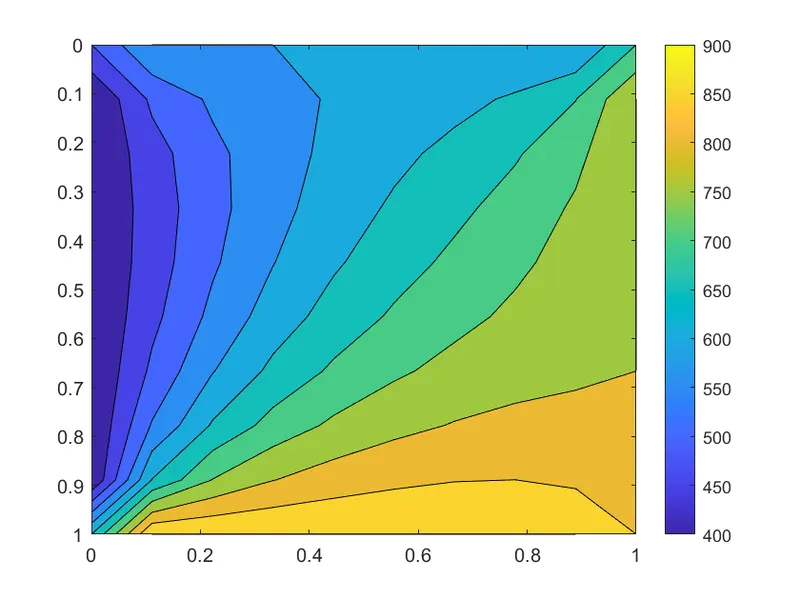
The programme worked as planned.
The temperature distribution plot is the same whether the conditions are steady or not.
Because the solution is also getting close to steady-state in transient analysis.
The top, bottom, left, and right sides of the graphs show the conditions at each of their edges.
The 3 iterative techniques are compared based on how many steps it takes to get to the solution.
Successive over-relaxation reduces the number of iterations in both steady and transient analysis.
The number of iterations taken by Successive over relaxaton, Gauss-Siedel, and Jacobi.
Reference:
Week 5.1 - Midterm project - Solving the steady and unsteady 2D heat conduction problem\ Assignment Help Video.
Week 5.1 - Midterm project - Solving the steady and unsteady 2D heat conduction problem\ Assignment Help Video.