Week 5.1 - Mid term project - Solving the steady and unsteady 2D heat conduction problem
NUMERICAL ANALYSIS OF 2-DIMENSIONAL HEAT CONDUCTION EQUATION
AIM:
To write a code to solve 2-Dimensional Heat conduction equation for Steady state analysis and Transient State Analysis using point iterative technique.
OBJECTIVE:
- To solve 2-Dimensional Heat conduction equation for,
(1). Steady state analysis
(2). Transient State Analysis.
- To implement the iterative methods (Jacobi, Gauss Seidal, Successive Over Realaxation SOR Methods) for solving implicit equations.
- To write code for implicit and explicit schemes for transient state analysis.
GIVEN DATA'S:
BOUNDARY CONDITIONS:
- Top Boundary = 600 K
- Bottom Boundary = 900 K
- Left Boundary = 400 K
- Right Boundary = 800 K
ITERATIVE METHODS:
1. Jacobi Method
2. Gauss-seidel Method
3. Successive over-relaxation (SOR) Method
INTRODCUTION:
DISCRETIZATION:
Discretization methods are used to divide the region of a continuous function i.e., the real solution to a system of differential equations into a discrete function, where the solution values are defined at each point in space and time. Discretization simply refers to the spacing between each point in solution space and then replace derivatives in the governing equation with difference quotients.
FINITE DIFFERENCE METHOD:
In numerical analysis, finite-difference methods (FDM) are a class of numerical techniques for solving differential equations by approximating derivatives with finite differences. Based on finite differences, it gives the numerical solutions for the values at discrete points in the domain which are known as grid points.
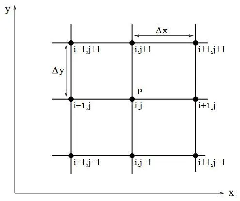
Finite differences method are used to compute approximate derivatives. This is used in numerical analysis in numerical ordinary differential equations and numerical partial differential equations, which gives the numerical solution of ordinary and partial differential equations respectively. The resulting methods are called finite-difference methods. Finite difference representations of derivatives are derived from Taylor series expansions.
POINT ITERATIVE TECHNIQUE:
An iterative method uses an initial value to generate a sequence of improving approximate solutions for a class of problems, in which the n-th approximation is derived from the previous ones. A specific implementation of an iterative method, including the termination criteria, is an algorithm of the iterative method. An iterative method is called convergent if the corresponding sequence converges for given initial approximations.
STEADY STATE ANALYSIS OF 2-D HEAT CONDUCTION EQUATION
TWO - DIMENSIONAL STEADY STATE HEAT CONDUCTION EQUATION:
The steady state Two -Dimensional Heat Conduction Equation,
`(del^2T)/(∂x^2)+(del^2T)/(∂y^2)=0` ................... (1)
`∇^2T=0` (Laplacian Equation)
This is the second order partial differential equation. Laplace's equation are in the simplest form of elliptic partial differential equation.
To discretize this second order partial differential equation in space along (x & y axis) to use the Central Difference scheme for space derivative. The partial derivative can be approximated using the derivative definition will be applied for space.
`(del^2T)/(del x^2)= (T_(i+1,j)-2T_(i,j)+T_(i-1,j))/(dx^2)` ...........(2)
`(del^2T)/(del y^2)= (T_(i,j+1)-2T_(i,j)+T_(i,j-1))/(dy^2)` ...........(3)
Substituting Equation (2) & (3) in equation (1),
`(T_(i+1,j)-2T_(i,j)+T_(i-1,j))/(dx^2) +(T_(i,j+1)-2T_(i,j)+T_(i,j-1))/(dy^2)=0`
Rearranging the Equation,
`(2T_(i,j))/(dx^2)+(2T_(i,j))/(dy^2) = (T_(i+1,j)+T_(i-1,j))/(dx^2) +(T_(i,j+1)+T_(i,j-1))/(dy^2)`
Simpliyfying the equation by considering,
T(i,j) = T_p
T(i+1,j) = T_R
T(i-1,j) = T_L
T(i,j+1) = T_T
T(i,j-1) = T_B
`T_p[(2((dx^2)+(dy^2)))/((dx^2)*(dy^2))] = (T_R+T_L)/(dx^2) +(T_T+T_B)/(dy^2)`
Considering K= `(2(dx^2)+(dy^2))/((dx^2)*(dy^2))`
Rearranging the Equations,
`T_p =(1/k) (T_R+T_L)/(dx^2) +(1/k)(T_T+T_B)/(dy^2)`
The Two-Dimensional Steady State Heat Conduction Equation,
`T_(i,j)=(1/k)(T_(i+1,j)+T_(i-1,j))/(dx^2) +(1/k)(T_(i,j+1)+T_(i,j-1))/(dy^2)`
(or)
`T_(i,j)=(1/k)[(T_(i+1,j)+T_(i-1,j))/(dx^2) +(T_(i,j+1)+T_(i,j-1))/(dy^2)]`
STEPS INVOLVED IN PROGRAMMING:
STEP 1: Defining the input parameters for the domain.
STEP 2: Defining the distance to the number of nodes provided.
STEP 3: Assigning the Initial Temperature to the respective number of nodes .
STEP 4: Applying Boundary conditions to the Left, Right, Top and Bottom of the domain and assigning to the corner nodes.
STEP 6: Updating the Initial and old Temperature values.
STEP7: Creating a function to Compute the Iterative methods.
STEP 8: Using the iterative method (Jacobi, Gauss seidal and SOR method)to determine the Temperature distribution at steady state for the respective number of nodes.
STEP 9: Updating the current temperature Value.
STEP 10: Calling a function to detrmine the Temperature distribution @ steady state.
STEP 12: Using contourf, the temperature distribution are potted for x and y Direction.
CODING:
FUNCTION FILE:
% Creating a function to solve Iterative Methods,
function [T,iteration]=Iterative_solver(tol,error,It_s,nx,ny,T_old,T,dx,dy,k)
  iteration=0;
   switch It_s     % Switching to Iterative Methods
       %% Solving Using Jacobi Method,
       case 1
     while(error>tol)           % Convergence loop
               for i=2:nx-1     % Spacial loop on x
                   for j=2:ny-1 % spacial loop on y
                       H=(T_old(i-1,j)+T_old(i+1,j))/(dx^2);
                       V=(T_old(i,j-1)+T_old(i,j+1))/(dy^2);
                       T(i,j)=k*(H+V);
                  end
              end
          error=max(max(abs(T-T_old)));
          T_old=T;    % Updating Temperature
          iteration=iteration+1;
     end
      %% Solving Using Gauss Seidal method,
     case 2
     while(error>tol)           % Convergence loop
               for i=2:nx-1     % Spacial loop on x
                   for j=2:ny-1 % spacial loop on y
                      H=(T(i-1,j)+T_old(i+1,j))/(dx^2);
                      V=(T(i,j-1)+T_old(i,j+1))/(dy^2);
                      T(i,j)=k*(H+V);
                  end
              end
          error=max(max(abs(T-T_old)));
          T_old=T;   % Updating Temperature
          iteration=iteration+1;
     end
     %% Solving Using Successive Over Relaxation Method (SOR),
     case 3
     omega=1.5;
     while(error>tol)           % Convergence loop
               for i=2:nx-1     % Spacial loop on x
                   for j=2:ny-1 % spacial loop on y
                      H=(T(i-1,j)+T_old(i+1,j))/(dx^2);
                      V=(T(i,j-1)+T_old(i,j+1))/(dy^2);
                      T(i,j)=k*(H+V);
                      T(i,j)=T_old(i,j)*(1-omega)+(omega*T(i,j));
                  end
              end
          error=max(max(abs(T-T_old)));
          T_old=T;   % Updating Temperature
          iteration=iteration+1;
     end
   end
end
M-CODE:
%% Solving 2-D Temperature Heat Conduction Equation,
% Steady State Heat Conduction Equation,
clear all;close all;clc
%% Inputting the parameters for Domain,
l=1;      % Length of the domain
nx=40;    % Number of Nodes on X -Axis
ny=nx;    % Number of Nodes on y -Axis
% Defining the length of domain repect to number of nodes,
x=linspace(0,l,nx);
y=linspace(0,l,ny);
% Finding the Grid Size along x and y axis,
dx=x(2)-x(1);  % Along X-axis
dy=y(2)-y(1);  % Along Y-axis
%% Defining the Temperature,
T_i=250;    % Initial condition for Temperature
T=T_i*ones(nx,ny);
% Applying Boundary Conditions,
T_L=400;
T_T=600;
T_R=800;
T_B=900;
% Assigning Boundary Conditions on Nodes,
T(1,:)=600;      % Temperature on Top
T(end,:)=900;    % Temperature on Bottom
T(:,1)=400;      % Temperature on Left
T(:,end)=800;    % Temperature on Right
% Assigning Average Temperature on Corner Grids,
T(1,1)=(T_L+T_T)/2;
T(1,ny)=(T_R+T_T)/2;
T(nx,1)=(T_L+T_B)/2;
T(nx,ny)=(T_B+T_R)/2;
% Updating the Temperature,
T_old=T;
% Defining Error & Tolerance;
tol=1e-4;   % Tolerence
error=1e5;  % Error
It_s=1:3;   % For Different Iterative Schemes (Jcobo - 1, Gauss Seidal- 2, SOR - 3)
% Calculation
k=(dx^2*dy^2)/(2*(dx^2+dy^2));
%% Calling a function to solve Iterative Solvers,
[T_J,iteration_jacobi]=Iterative_solver(tol,error,It_s(1),nx,ny,T_old,T,dx,dy,k);  % Calling Jacobi Method
[T_GS,iteration_GS]=Iterative_solver(tol,error,It_s(2),nx,ny,T_old,T,dx,dy,k);     % Calling Gauss Seidal Method
[T_SOR,iteration_SOR]=Iterative_solver(tol,error,It_s(3),nx,ny,T_old,T,dx,dy,k);   % Calling SOR Method

%% Plotting,
% Plotting for Temperature Distribution by Jacobi Method
figure("Name",'STEADY STATE ANALYSIS')
contourf(x,y,T_J,'ShowText','on','LineWidth',0.5);
colorbar
colormap(jet)
set(gca,'YDir','reverse')
text_title=({'2-DSteady State Heat Conduction (Jacobi Method)';['No.of.Grid Points =',num2str(nx)];['Total Iterations =',num2str(iteration_jacobi)]});
title(text_title)
xlabel('X-Direction')
ylabel('Y-Direction')

% Plotting for Temperature Distribution by Gauss Seidal Method
figure("Name",'STEADY STATE ANALYSIS')
contourf(x,y,T_GS,'ShowText','on','LineWidth',0.5);
colorbar
colormap(jet)
set(gca,'YDir','reverse')
text_title=({'2-D Steady State Heat Conduction (Gauss Seidal Method)';['No.of.Grid Points =',num2str(nx)];['Total Iterations =',num2str(iteration_GS)]});
title(text_title)
xlabel('X-Direction')
ylabel('Y-Direction')

% Plotting for Temperature Distribution by Successive Over Relaxation (SOR) Method
figure("Name",'STEADY STATE ANALYSIS')
contourf(x,y,T_SOR,'ShowText','on','LineWidth',0.5);
colorbar
colormap(jet)
set(gca,'YDir','reverse')
text_title=({'2-D Steady State Heat Conduction (SOR Method)';['No.of.Grid Points =',num2str(nx)];['Total Iterations =',num2str(iteration_SOR)]});
title(text_title)
xlabel('X-Direction')
ylabel('Y-Direction')
CODING EXPLANATION:
- Inputting the Domain parameters for length.
- Assigning the number of nodes on x and y axis as (nx and ny) respectively, based on the number of nodes the array for the x-axis abd y-axis are assigned to the length of the domain using linspace command, equal intervels of arrays are created over the domain length.
- Determining the distance between the two nodes dx and dy , by differncing the second node to the first node.
`dx=x(2) -x(1) or dx=l/(nx-1)` and `dx=y(2) -y(1) or dy=l/(ny-1)`
- Defining the initial temperature values to the number of repective nodes using ones command. Ones command creating the value of one to the respective number of nodes.
- Applying Boundary conditions on top, bottom, left and right side of the domain using the respective commands and the corner node temperature are assigned by averaging the temperature on the nearby nodes.
- Updating the initial and old temperature values.
- Defining the error and tolerance creteria as 1e-4.
- Creating a function to solve iterative methods (Jacobi, Gauss seidal and SOR method) by passing the inputs as, tolerence, error, nx,ny,Temperature values and calculated terms.
- In the function the iterative methods are done using the convergence and nodel loops.
- The Switch case command is used to iterate for different methods based on given inputs respectively.
- The convergence loop- while loop is used to perform the error and tolerence which exceeds the numeric solutions are close to the exact solutions.
- For 2-D two for loops are assigned to perform nodel iterations on x and y axis.
- The error are determined for the iterated temperature values and the Temperatures values are updated.
- Using Iteration counter the number of iterations are counted for all the three iterative methods.
- By calling a function the temperature distribution for the different iterative methods are computed and plotted accordingly.
- Plotting the Temperature distrbution profiles for the respective number of time step's dt for the domain along x and y axis.
- Using Contourf command the temperature distribution for the respectieve number of nodal points are plotted.
PLOTTING:
- JACOBI ITERATIVE METHOD:-
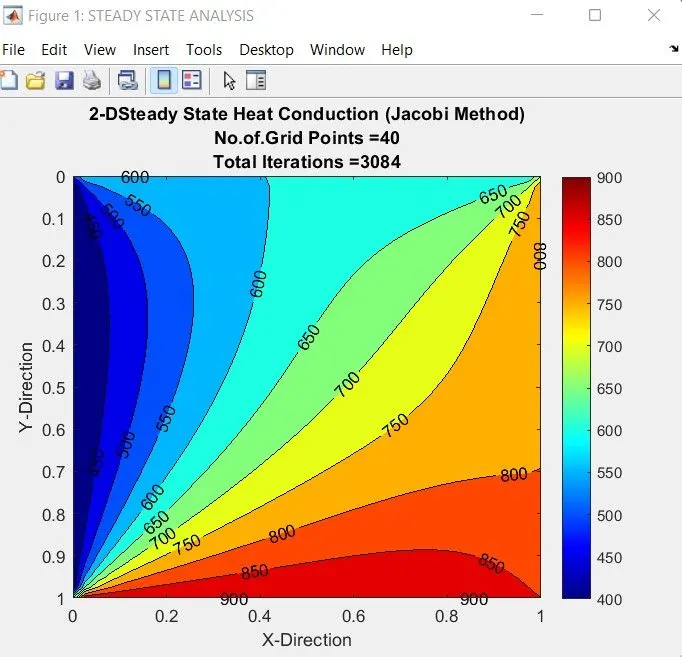
- The plotting describes, Temperature distribution along x and y axis for the steady state analysis of 2-D heat conduction equation.
- From the plotting the temperature at the bottom of domain as the higher temperature can be distributed over the domain.
- The Jacobi Iterative method are performed for steady state analysis and for 3084 iterations are required to get the convergence of steady state for the domain.
2. GAUSS SEIDAL ITERATIVE METHOD:-
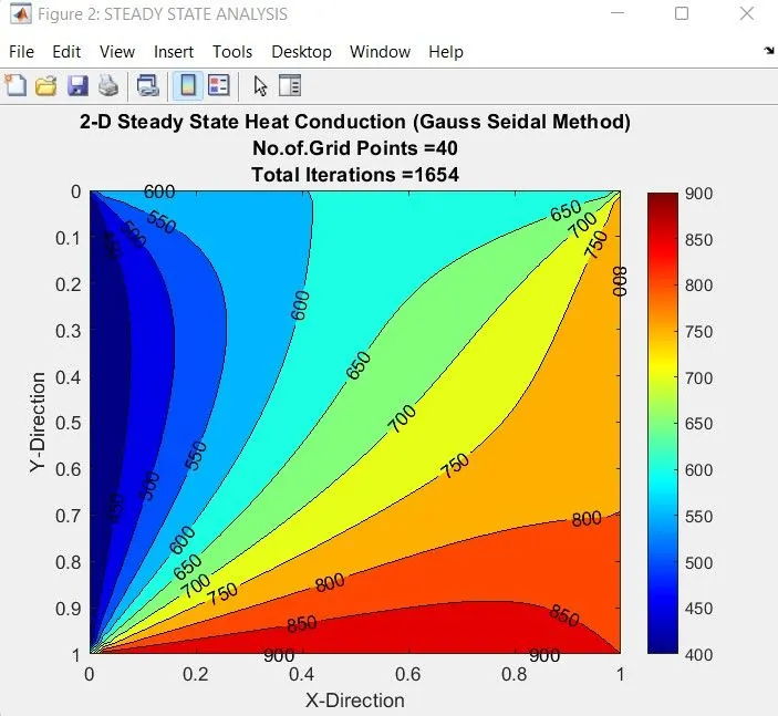
- The plotting describes, Temperature distribution along x and y axis for the steady state analysis of 2-D heat conduction equation.
- From the plotting the temperature at the bottom of domain as the higher temperature can be distributed over the x and y co-ordinates of a domain.
- The Gauss seidal Iterative method are performed for steady state analysis and for 1654 iterations are required to get the convergence of steady state for the domain.
- Compared to Jacobi method, the gauss seidal method converge faster.
3. SUCCESSIVE OVER RELAXATION METHOD:-
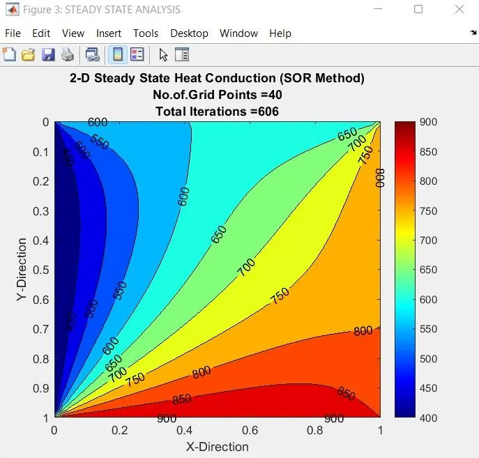
- The plotting describes, Temperature distribution along x and y axis for the steady state analysis of 2-D heat conduction equation.
- From the plotting the temperature at the bottom of domain as the higher temperature can be distributed over the x and y co-ordinates of a domain.
- The Successive over relaxation iterative method are performed for steady state analysis and for 606 iterations are required to get the convergence of steady state for the domain.
- Compared to Jacobi method and gauss seidal method the SOR iterative method converge faster.
TRANSIENT STATE ANALYSIS OF 2-D HEAT CONDUCTION EQUATION
TRANSIENT STATE:
The Two -Dimensional Transient Heat Conduction eqaution is,
`(delT)/(delt)=alpha*[(∂^2T)/(∂x^2)+(∂^2T)/(∂y^2)]` .............. (1)
This is the second order partial differential equation. Laplace's equation are in the simplest form of elliptic partial differential equation and time dependent partial differential equation.
To discretize this equation in space and time to use the Forward Difference scheme for time derivative and Central Difference scheme for space derivative. The partial derivative can be approximated using the derivative definition will be applied both for space and time;
Here the terms represents,
`(del T)/ (delt)` = Time Derivative Term
`[(∂^2T)/(∂x^2)+(∂^2T)/(∂y^2)] = Space Derivative Ter`
`alpha` = Termal Diffusivity
TIME DERIVATIVE:
Applying Forward difference scheme for the time derivative;
`(del T)/ (delt) = (T_(i,j)^(n+1)-T_(i,j)^n)/(△t)` ................ (2)
SPACE DERIVATIVE:
Applying Central differencing for the space term
`(del^2T)/(del x^2)= (T_(i+1,j)-2T_(i,j)+T_(i-1,j))/(dx^2)`.............. (3)
`(del^2T)/(del y^2)= (T_(i,j+1)-2T_(i,j)+T_(i,j-1))/(dy^2)`............ (4)
Substituting equation (2), (3) & (4) in equation (1),
`(T_(i,j)^(n+1)-T_(i,j)^n)/(△t) =alpha *[ (T_(i+1,j)-2T_(i,j)+T_(i-1,j))/(dx^2)+(T_(i,j+1)-2T_(i,j)+T_(i,j-1))/(dy^2)]^n`
Rearranging the Equation;
`T_(i,j)^(n+1)=T_(i,j)^n+ alpha*((Deltat)/(dx^2)) * (T_(i+1,j)-2T_(i,j)+T_(i-1,j))+alpha*((Deltat)/(dy^2)) *(T_(i,j+1)-2T_(i,j)+T_(i,j-1))]^n`
Considering,
K1 = `alpha*((Deltat)/(dx^2))`
k2= `alpha*((Deltat)/(dy^2))`
`T_(i,j)^(n+1)=T_(i,j)^n+ [(K1) * (T_(i+1,j)-2T_(i,j)+T_(i-1,j))+(K2) *(T_(i,j+1)-2T_(i,j)+T_(i,j-1))]^n`
where n+1 and n are two consecutive steps in time and i,j are neighbouring points of the discretized x an Y - coordinate (grid points). The only unknown in the equation written in this way is `Ti^(n+1)`.To solve for this unknown to get an equation that allows us to advance in time as Time Marching Procedure Method. This equation is used in program to solve the 2-D Heat conduction equation numerically.
EXPLICIT AND IMPLICIT METHOD:
- The explicit method and implicit method are numerical analysis methods used to solve a time-dependent differential equation.
- The explicit method calculates the system status at a future time from the currently known system status.
(ie;), if know the state at n, can calculate the state at n+1.
- In explicit method the stability is so low that need to use a step size small enough to prevent divergence.
- The implicit method calculates the system status at a future time from the system statuses at present and future times.
- The implicit method has high stability and converges if setted with proper parameters.
- As the implicit method can use a sufficiently large step size, it is suitable for solving equations that involve a long time.
- Also, in non-linear equations such as contact, it is difficult to predict a future from the past state.
EXPLICIT EQUATION:-
`T_(i,j)^(n+1)=T_(i,j)^n+ [(K1) * (T_(i+1,j)-2T_(i,j)+T_(i-1,j))+(K2) *(T_(i,j+1)-2T_(i,j)+T_(i,j-1))]^n`
Simply,
`T_p^(n+1)=T_p^n+ [(K1) * (T_R-2T_P+T_L)+(K2) *(T_T-2T_P+T_B)]^n`
IMPLICIT EQUATION:
`T_(i,j)^(n+1)=T_(i,j)^n+ [(K1) * (T_(i+1,j)-2T_(i,j)+T_(i-1,j))+(K2) *(T_(i,j+1)-2T_(i,j)+T_(i,j-1))]^(n+1)`
Rearranging the Equation,
`T_(i,j)^(n+1)=(T_(i,j)^n+ (K1) * (T_(i+1,j)+T_(i-1,j))+(K2) *(T_(i,j+1)+T_(i,j-1))^(n+1))/(1+(2*(k1+k2))`
COURANT NUMBER:
The Courant-Friedrichs-Lewy (CFL) condition is absolutely essential in solving the partial differential equations. This non dimensionless number arises while solving the time marching problems. It expresses that the distance that any information travels during the time step length within the mesh must be lower than the distance between mesh elements.
In other words, information from a given cell or mesh element must propagate only to its immediate neighbors. The derivation of the CFL condition leads to the formula for Courant number and is given by,
`CFL=alpha*(Δt)/(Δx^2) <=0.25 ; alpha*(Δt)/(Δy^2) <=0.25`
Where,
CFL = Courant number, u
α = Thermal Diffusivity
Δt = Time step size
Δx = The length between mesh elements.
When the Courant number exceeds the value of 0.5 for Heat conduction equation the solution will be unstable and blew off, instabilities are amplified throughout the domain and may cause divergence of the simulation.
`CFL=alpha*(Δt)[1/(Δx^2) +1/(Δy^2)]<=0.5`
Courant number can be controlled by altering the time or space interval. When the space interval is reduced or time interval is increased the courant number increases. Since courant number governs the stability of a problem in an explicit method it is very important to choose the intervals precisely.
STEPS INVOLVED IN PROGRAMMING:
STEP 1: Defining the input parameters for the domain.
STEP 2: Defining the distance to the number of nodes provided.
STEP 3: Assigning the Initial Temperature to the respective number of nodes .
STEP 4: Applying Boundary conditions to the Left, Right, Top and Bottom of the domain and assigning to the corner nodes.
STEP 6: Updating the Previous and old Temperature values.
STEP7: Computing Transient state 2-D heat conduction equation explicitlly.
STEP8: Computing Transient state 2-D heat conduction equation Implicitlly.
STEP 9: Using the iterative method (Jacobi, Gauss seidal and SOR method)to determine the Temperature distribution at Transient state for the respective number of nodes.
STEP 10: Updating the temperature Value and Previous time step values of temperature.
STEP 11: Using contourf, the temperature distribution are potted for x and y Direction.
CODING FOR NUMERICAL ANALYSIS OF 2-DIMENSIONAL TRANSIENT HEAT CONDUCTION EQUATION:
(1). EXPLCIT METHOD:
M-CODE:
%% Solving 2-D Temperature Heat Conduction Equation,
% Transient Heat Conduction Equation, By Using Explicit Method,
clear all;close all;clc
% Inputting the parameters for Domain,
l=1;      % Length of the domain
nx=40;    % Number of Nodes on X -Axis
ny=nx;    % Number of Nodes on y -Axis
% Defining the length of domain repect to number of nodes,
x=linspace(0,l,nx);   % Along X-Direction
y=linspace(0,l,ny);   % Along Y- Direction
% Finding the Grid Size along x and y axis,
dx=x(2)-x(1);
dy=y(2)-y(1);
% Defining the Initial Temperature,
T_i=250;           % Initial condition for Temperature
T=T_i*ones(nx,ny); % Assigning Temperature on nodes
% Applying Boundary Conditions,
T_L=400;        % Temperature on the Left
T_T=600;        % Temperature on the TOP
T_R=800;        % Temperature on the RIGHT
T_B=900;        % Temperature on the BOTTOM
% Assigning Boundary Conditions on Nodes,
T(1,:)=600;      % Temperature on Top
T(end,:)=900;    % Temperature on Bottom
T(:,1)=400;      % Temperature on Left
T(:,end)=800;    % Temperature on Right
% Assigning Average Temperature on Corner Grids,
T(1,1)=(T_L+T_T)/2;
T(1,ny)=(T_R+T_T)/2;
T(nx,1)=(T_L+T_B)/2;
T(nx,ny)=(T_B+T_R)/2;
% Updating the current Temperature,
T_old=T;
% Defining the Time Steps
t=0.15;     % Time for Temperature Distribution
dt=1e-4;    % Time steps
nt=t/dt;    % Number of Time Steps
alpha=1.4;  % Thermal Diffusivity
% Calculations,
k1=alpha*(dt/dx^2);
k2=alpha*(dt/dy^2);
CFL=k1+k2;
%% TIME MARCHING PROCEDURE,
   Iteration=1;
   for k=1:nt    % Time loop
        for i=2:nx-1      % Space loop
            for j=2:ny-1  % Space loop
                H=(T_old(i+1,j)-2*T(i,j)+T_old(i-1,j));
                V=(T_old(i,j+1)-2*T(i,j)+T_old(i,j-1));
                T(i,j)=T_old(i,j)+k1*(H)+k2*(V);
            end
        end
        T_old=T;
        Iteration=Iteration+1;
   end
 %% PLOTTING FOR EXPLICIT METHOD
figure('Name','TRANSIENT STATE ANALYSIS - EXPLICIT')
contourf(x,y,T,'ShowText','on','LineWidth',0.5);
colorbar
colormap(jet)
set(gca,'YDir','reverse')
title('2-D Transient State Heat Conduction (Explicit Method)')
text=sprintf(['Total Iterations =%d;  ','CFL=%g\n   ','Grid Points=%g;  ','dt=%g;  ','dx=%g'],...
              Iteration,CFL,nx,dt,dx);
subtitle(text)
xlabel('X-Direction')
ylabel('Y-Direction')
PLOTTING:
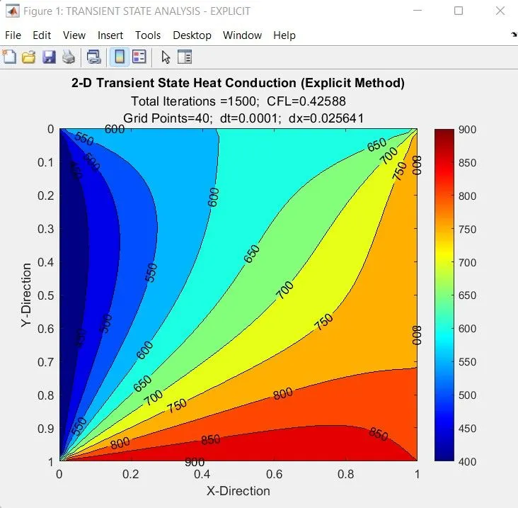
- The plotting describes, Temperature distribution along x and y axis for the Transient state analysis of 2-D heat conduction equation.
- From the plotting the temperature at the bottom of domain as the higher temperature can be distributed over the x and y co-ordinates of a domain.
- The Explicit method are performed for Transient state analysis and for 1500 iterations are performed to get the convergence of steady state for the domain @ time step of 1e-4 @ dx= 0.02564.
- The CFL creteria for the Explicit method plays crucial role in the stability of the solution.
- If the CFL values exceeds 0.5 the solution will be unstable based on the respective time step.
(2). IMPLICT METHOD:-
- The implicit method calculates the system status at a future time from the system state at present and future times.
- The implicit method has high stability and converges if setted with proper parameters.
- As the implicit method can use a sufficiently large step size, it is suitable for solving equations that involve a long time.
- The implicit methods are insensitive with changes in courant number (C).
M-CODE:
%% Solving 2-Dimensional Temperature Heat Conduction Equation,
% Transient Heat Conduction Equation, By Using Implicit Method,
clear all;close all;clc
%% Inputting the Domain Parmeters,
l=1;      % Length of the domain
nx=40;    % Number of Nodes on X -Axis
ny=nx;    % Number of Nodes on y -Axis
% Defining the length of domain repect to number of nodes,
x=linspace(0,l,nx);
y=linspace(0,l,ny);
% Finding the Grid Size along x and y axis,
dx=x(2)-x(1);   % On X-axis
dy=y(2)-y(1);   % on Y-axis
%% Defining the Initial Temperature,
T_i=250;           % Initial condition for Temperature
T=T_i*ones(nx,ny); % Assigning Temperature on nodes
% Applying Boundary Conditions,
T_L=400;        % Temperature on the Left
T_T=600;        % Temperature on the TOP
T_R=800;        % Temperature on the RIGHT
T_B=900;        % Temperature on the BOTTOM
% Assigning Boundary Conditions on Nodes,
T(1,:)=600;      % Temperature on Top
T(end,:)=900;    % Temperature on Bottom
T(:,1)=400;      % Temperature on Left
T(:,end)=800;    % Temperature on Right
% Assigning Average Temperature on Corner Grids,
T(1,1)=(T_L+T_T)/2;
T(1,ny)=(T_R+T_T)/2;
T(nx,1)=(T_L+T_B)/2;
T(nx,ny)=(T_B+T_R)/2;
% Updating the Temperatures,
T_old=T;
T_prev=T;
% Defining the Time Steps
t=0.2;     % Time for Temperature Distribution
dt=1e-4;    % Time steps
nt=t/dt;    % Number of Time Steps
alpha=1.4;  % Thermal Diffusivity
% Calculations,
k1=alpha*(dt/dx^2);
k2=alpha*(dt/dy^2);
CFL=k1+k2;
Term1=1/(1+(2*(k1+k2)));
Term2=k1*Term1;
Term3=k2*Term1;
% Defining the Tolerence,
tol=1e-4;     % Tolerence Creteria
omega=1.2;    % Relaxation Factor
Iteration=1;  % Initial Iteration
%% Input User Selection Prompt,
prompt=(['Select Iterative Method\n (1).JACOBI ITERATIVE METHOD\n ' ...
    '(2).GAUSS SEIDAL ITERATIVE METHOD\n ' ...
    '(3).SOR ITERATIVE METHOD\n']);
Iterative_Method=input(prompt);
%% Solving 2-D Using Iterative Method,
% Time loop,
tic
for k=1:nt
   error=1e5;     % Initialize Error on each iteration time loop
   if Iterative_Method==1    %% Jacobi Iterative Method
    % Convergence loop
    while error>tol
        % Nodal loop
        for i=2:nx-1
            for j=2:ny-1
                 H=(T_old(i+1,j)+T_old(i-1,j));
                 V=(T_old(i,j+1)+T_old(i,j-1));
                 T(i,j)=((T_prev(i,j)*Term1)+(Term2*H)+(Term3*V));
            end
        end
        error=max(max(abs(T-T_old)));
        % Updating temperatures,
        T_old=T;
        Iteration=Iteration+1;
    end
  end
%% Gauss Seidal Iterative Method
if Iterative_Method==2
    % Convergence loop
    while error>tol
        % Nodal loop
        for i=2:nx-1
            for j=2:ny-1
                 H=(T_old(i+1,j)+T(i-1,j));
                 V=(T_old(i,j+1)+T(i,j-1));
                 T(i,j)=((T_prev(i,j)*Term1)+(Term2*H)+(Term3*V));
            end
        end
        error=max(max(abs(T-T_old)));
        % Updating temperatures,
        T_old=T;
        Iteration=Iteration+1;
    end
end
%% Successive Over Relaxation (SOR) Iterative Method
   if Iterative_Method==3
    % Convergence loop
    while error>tol
        % Nodal loop
        for i=2:nx-1
            for j=2:ny-1
                 H=(T(i-1,j)+T_old(i+1,j));
                 V=(T(i,j-1)+T_old(i,j+1));
                 T(i,j)=((T_prev(i,j)*Term1)+(Term2*H)+(Term3*V));
                 T(i,j)=(T_old(i,j)*(1-omega))+omega*T(i,j);
            end
        end
        error=max(max(abs(T-T_old)));
        % Updating temperatures,
        T_old=T;
        Iteration=Iteration+1;
    end
   end
    T_prev=T;
    sim_time_Jacobi=toc;   % Simulation time for Jacobi Iteration
    sim_time_Gs=toc;       % Simulation time for Gauss seidal Iteration
    sim_time_SOR=toc;      % Simulation time for SOR Iteration

%% Plotting
figure(1)
contourf(x,y,T,'ShowText','on','LineWidth',0.5)
colorbar
colormap('jet')
set(gca,'YDir','reverse')
    if Iterative_Method==1
    title('2-D Transient State Heat Conduction (Implicit - Jacobi Method)')
    text=sprintf(['Total Iterations =%d;  ','CFL=%g\n   ','Grid Points=%g;  ','dt=%g;  ','dx=%g\n','Simulation Time=%g'],...
                  Iteration,CFL,nx,dt,dx,sim_time_Jacobi);
    subtitle(text)
    elseif Iterative_Method==2
    title('2-D Transient State Heat Conduction (Implicit - Gauss Seidal Method)')
    text=sprintf(['Total Iterations =%d;  ','CFL=%g\n   ','Grid Points=%g;  ','dt=%g;  ','dx=%g\n','Simulation Time=%g'],...
                  Iteration,CFL,nx,dt,dx,sim_time_Gs);
    subtitle(text)
    elseif Iterative_Method==3
    title('2-D Transient State Heat Conduction (Implicit - SOR Method)')
    text=sprintf(['Total Iterations =%d;  ','CFL=%g\n   ','Grid Points=%g;  ','dt=%g;  ','dx=%g\n','Simulation Time=%g'],...
                  Iteration,CFL,nx,dt,dx,sim_time_SOR);
    subtitle(text)
    end
xlabel('X-Direction')
ylabel('Y-Direction')
end
CODING EXPLANATION:
- Inputting the Domain parameters for length.
- Assigning the number of nodes on x and y axis as (nx and ny) respectively, based on the number of nodes the array for the x-axis abd y-axis are assigned to the length of the domain using linspace command, equal intervels of arrays are created over the domain length.
- Determining the distance between the two nodes dx and dy , by differncing the second node to the first node.
`dx=x(2) -x(1) or dx=l/(nx-1)` and `dx=y(2) -y(1) or dy=l/(ny-1)`
- Defining the initial temperature values to the number of repective nodes using ones command. Ones command creating the value of one to the respective number of nodes.
- Applying Boundary conditions on top, bottom, left and right side of the domain using the respective commands and the corner node temperature are assigned by averaging the temperature on the nearby nodes.
- Updating the initial and old temperature values.
- Defining the error and tolerance creteria as 1e-4.
- Defining the time steps to solve the temperature distribution from transient state to steady state for convergence of the solution.
- Assigning the thermal diffusivity value and relaxation factor to solve the iterative methods (Jacobi, Gauss seidal and Successive over relaxation Methods) numerically.
SELECTION OF ITERATIVE METHOD:
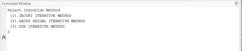
- Based on the selection the respective iterative methods are selected and computed accordingly.
- Using Time marching method the Explicit method for 2-D heat conduction eqaution are analyzed numerically and updating the temperatire values.
- Determinig the Number of time steps (nt) by using the simulation run time for the respective time steps.
- Using "for" loop the time step (dt) are iterated for varying number of time steps.
- Using the Forward Differencing approximations the time derivatives are derived.
- Using the Central Diferencing approximations the space derivatives are derived along x and y axis.
- By combing the time and space derivatives the respective the future time step for the respective temperature distribution for the domain's are determined.
- By using the "for" loop the time loop are iterated with to the respective space loop for the respective nodes.
- After the space loop iterted, updating the Temperatures for the repective time and space loop.
- Computing the simulation time for each iteration on time steps using "Tic Toc" command tic works with the toc function to measure elapsed time.
- The tic function records the current time, and the toc function uses the recorded value to calculate the elapsed time.
- Plotting the Temperature distrbution profiles for the respective number of time step's (dt's) to the number of iterations.
- Using Contourf command the temperature distribution for the respectieve number of nodal points are plotted along x and y axis.
PLOTTING:
- JACOBI ITERATIVE METHOD:-
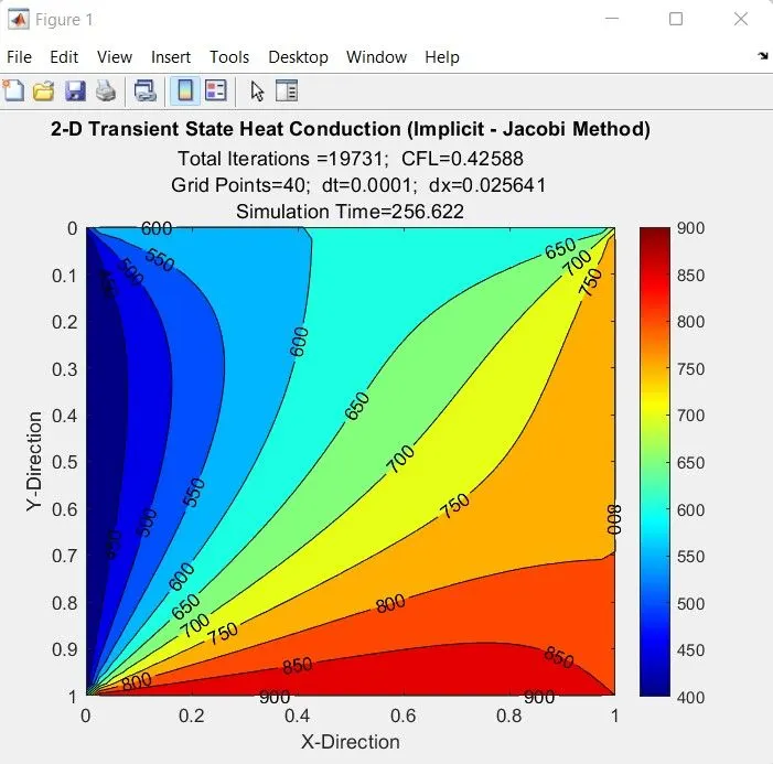
- The plotting describes, Temperature distribution along x and y axis for the Tarnsient state analysis of 2-D heat conduction equation implicitlly.
- From the plotting the temperature at the bottom of domain as the higher temperature can be distributed over the domain.
- The Jacobi Iterative method are performed for transient state analysis and for 19732 number of iterations are required to get the convergence of steady state for the domain.
- The convergence loop are performed under the time loop "nt" where the older value of temperature and previous time step values of temperature are updated accordingly.
- GAUSS SEIDAL ITERATIE METHOD:-
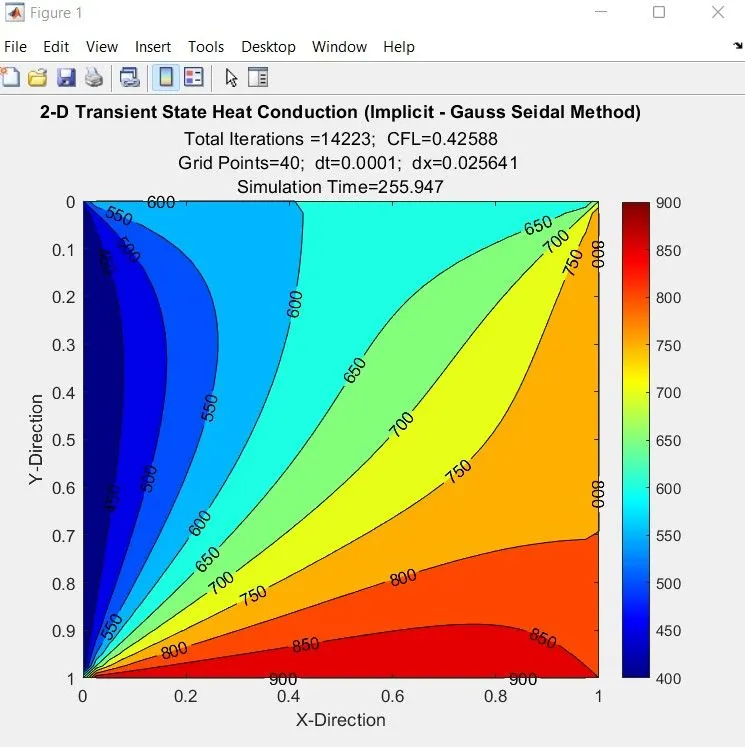
- The plotting describes, Temperature distribution along x and y axis for the Tarnsient state analysis of 2-D heat conduction equation implicitlly.
- From the plotting the temperature at the bottom of domain as the higher temperature can be distributed over the domain.
- The Gauss Seidal Iterative method are performed for transient state analysis and for 14223 number of iterations are required to get the convergence of steady state for the domain.
- The convergence loop are performed under the time loop "nt" where the older value of temperature and previous time step values of temperature are updated accordingly.
- Compared to Jacobi Iterative method the Gauss Seidal method converge faster.
- SUCCESSIVE OVER RELAXATION METHOD:-
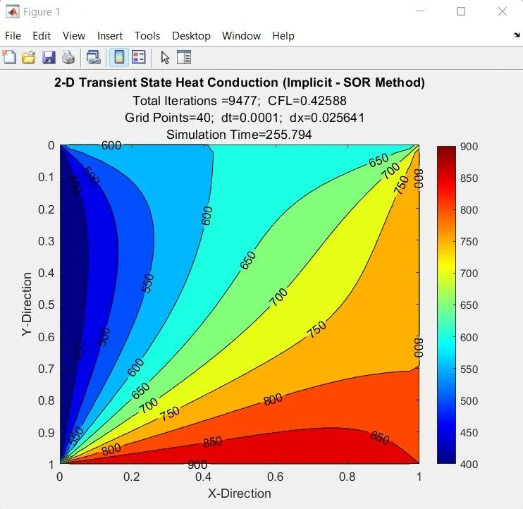
- The plotting describes, Temperature distribution along x and y axis for the Tarnsient state analysis of 2-D heat conduction equation implicitlly.
- From the plotting the temperature at the bottom of domain as the higher temperature can be distributed over the domain.
- The Successive Over Relaxation Iterative method are performed for transient state analysis and for 9477 number of iterations are required to get the convergence of steady state for the domain.
- The convergence loop are performed under the time loop "nt" where the older value of temperature and previous time step values of temperature are updated accordingly.
- Compared to Jacobi Iterative method and Gauss Seidal method, the SOR Iterative method converge faster based on the relaxation factor.
- The relaxation factor are considered as a certain range to get the solution converge faster then gauss seidal method.
M-CODE LINK:
CONCLUSION:
- The 2-Dimensional Steady state heat conduction equation are analyzed numerically by using iterrative methods (Jacobi, Gauss Saidel and Successive over Relaxation Methods).
- The 2-Dimensional Transient state heat conduction equation are analyzed numerically by Explicit and Implicit methods.
- The Thermal diffusivity value are selected as α">α=1.4 to diffuse the temperature distribution at transient heat conduction.
- The Relaxation factor ω">ω are selected as in the value of 1.2, if the relaxation factor overtunned in SOR method the iterations are overshotted then the targetted value and taking longer time of iterations and computation time then Gauss seidal method.
- The Transient and Steady state analysis of two Dimensional eat conduction equation are analyzed and the temperature distribution along the domian for the defined boundary conditions are performed.
- In steady state analysis the Number of iterations to converge for steady state for faster in SOR iterative method then Gauss Seidal Iterative metod then Jacobi method.
- In Transient state Explicit analysis the Equations are directly solved on the time loop to get the desired temperature distribution along x and y axis.
- In Transient state Implicit analysis the system of equtions are solved Using Iterative methods to get the convergence of the steady state solutions.