Week 5.1 - Mid term project - Solving the steady and unsteady 2D heat conduction problem

Aim

1. Steady state analysis & Transient State Analysis

Solve the 2D heat conduction equation by using the point iterative techniques. The Boundary conditions for the problem are as follows;

Top Boundary = 600 K

Bottom Boundary = 900 K

Left Boundary = 400 K

Right Boundary = 800 K

You will implement the following methods for solving implicit equations.

1. Jacobi

2. Gauss-seidel

3. Successive over-relaxation

Your absolute error criteria is 1e-4

2. write code for both implicit and explicit schemes (This is for the Transient Analysis only)

2D heat conduction equation

(∂^2 T)/(∂x^2 )+(∂^2 T)/(∂y^2 )=1/α (∂T)/(∂t)ddkjfvjdd

The heat conduction equation can be solved in two ways

1. Steady state

2. Transient state

A)Solving 2D steady state heat conduction equation

Here the time term gets eliminated ie, ∂T∂t=0∂T∂t=0

so the equation becomes,(∂^2 T)/(∂x^2 )+(∂^2 T)/(∂y^2 )=0

This equation is elliptic in nature so the information is taken from the surroundings,

hence we can write the equation as follows:

TL−2TP+TRΔx2+TT−2Tp+TBΔy2=0TL-2TP+TRΔx2+TT-2Tp+TBΔy2=0

if we put K =2Δx2+Δy2Δx2⋅Δy22Δx2+Δy2Δx2⋅Δy2

we can write the expression for TpTp from the above equation as:

Tp=1k(TL+TRΔx2+TT+TBΔy2)Tp=1k(TL+TRΔx2+TT+TBΔy2)

The above equation is used for iteration. There will three methods that I will be using here

1. Jacobi method

In numerical linear algebra, the Jacobi method is an iterative algorithm for determining the solutions of a strictly diagonally dominant system of linear equations. Each diagonal element is solved for, and an approximate value is plugged in. The process is then iterated until it converges.

2. Gauss Siedel method

Gauss-Seidel method is an iterative method to solve a set of linear equations and is very much similar to Jacobi’s method. This method is also known as the Liebmann method or the method of successive displacement. The name successive displacement is because the second unknown is determined from the first unknown in the current iteration, and the third unknown is determined from the first and second unknowns.

3. Successive over relaxed method

The method of successive over-relaxation (SOR) is a variant of the Gauss-Siedel method for solving a linear system of equations, resulting in faster convergence. A similar method can be used for any slowly converging iterative process

for converting into Matlab code' I've changed temperature terms as follows:

TpTp = T(i,j)

TLTL = T(i-1,j)

TRTR = T(i+1,j)

TBTB = T(i,j-1)

TTTT = T(i,j+)

• For Jacobi method all T on the right-hand side will be the old calculated values of T, Hence I'll be using Told
• For Gauss-Siedel method only updated values are to be substituted for T for the previous nodes but can use either T or Told for successive nodes
• And for successive over relaxed method, it will be of the form

T(i,j) = (1-w)*Told + w*(Tgs)

Tgs is the value found through gauss siedel method

here when omega, w >1 then it is known as over relaxed

and whe w<1 it will be under relaxed.

clear all
close all
clc

%inputs
L=1;
nx=20;
ny=20;
error= 9e9;
tol= 1e-4;

iteraction_method=2;

if iteraction_method == 1
    T_jacobian = jacobian_method(L,nx,ny,error,tol);
end

if iteraction_method == 2
    T_GS = GS_method(L,nx,ny,error,tol);
end

if iteraction_method == 3
    T_SOR= SOR_method(L,nx,ny,error,tol);
end

Code for steady state Jacobian

function [T_jacobian] = jacobian_method(L,nx,ny,error,tol);

tic

x=linspace(0,L,nx);
y=linspace(0,L,ny);
dx=(L/nx-1);
dy=(L/ny-1);

%temperature matrix
T=300*ones(nx,ny);

Tleft = 400;
Tright = 800;
Ttop = 600;
Tbottom = 900;

T(:,1)=Tleft;
T(1,:)=Ttop;
T(:,end)=Tright;
T(end,:)=Tbottom;

%defining the edge values
T(1,1) = (Ttop + Tleft)/2;
T(end,end) = (Tright+Tbottom)/2;
T(1,end) = (Ttop + Tright)/2;
T(end,1) = (Tbottom+Tleft)/2;


K=2*(dx^2+dy^2)/((dx^2)*(dy^2));

Told=T;
j_iter=1;

while (error>tol)
    for i=2:(nx-1)
        for j=2:(ny-1)
            T(i,j)=(1/K)*(((Told(i-1,j)+Told(i+1,j))/dx^2)+((Told(i,j-1)+Told(i,j+1))/dy^2));

        end
    end
    error=max(max(abs(Told-T)));
    Told=T;
    j_iter=j_iter+1;
end

%plotting
figure (1)

contourf(x,y,T)
colormap(jet)
colorbar

toc;

pause(0.03)
titletext=sprintf('Jacobian method with iteraction number =%d',j_iter);
title(titletext)
xlabel('x')
ylabel('y')
T_jacobian=T;
end

Code for steady state Gauss-siedel

function [T_GS] =GS_method(L,nx,ny,error,tol)


tic

x=linspace(0,L,nx);
y=linspace(0,L,ny);
dx=(L/nx-1);
dy=(L/ny-1);

%temperature matrix
T=300*ones(nx,ny);

Tleft = 400;
Tright = 800;
Ttop = 600;
Tbottom = 900;

T(:,1)=Tleft;
T(1,:)=Ttop;
T(:,end)=Tright;
T(end,:)=Tbottom;

%defining the edge values
T(1,1) = (Ttop + Tleft)/2;
T(end,end) = (Tright+Tbottom)/2;
T(1,end) = (Ttop + Tright)/2;
T(end,1) = (Tbottom+Tleft)/2;


K=2*(dx^2+dy^2)/((dx^2)*(dy^2));

Told=T;
GS_iter=1;

while (error>tol)
    for i=2:(nx-1)
        for j=2:(ny-1)
            T(i,j)=(1/K)*(((T(i-1,j)+T(i+1,j))/dx^2)+((T(i,j-1)+T(i,j+1))/dy^2));

        end
    end


end

error=max(max(abs(Told-T)));
Told=T;
GS_iter=GS_iter+1;


%plotting
figure (2)

contourf(x,y,T)
colormap(jet)
colorbar

toc;

pause(0.03)
titletext=sprintf('GS method with iteractin number =%d',GS_iter);
title(titletext)
xlabel('x')
ylabel('y')

T_GS=T;


end

Code for steady state SOR method

function [T_SOR] = SOR_method(L,nx,ny,error,tol)

tic

x=linspace(0,L,nx);
y=linspace(0,L,ny);
dx=(L/nx-1);
dy=(L/ny-1);

%temperature matrix
T=300*ones(nx,ny);

Tleft = 400;
Tright = 800;
Ttop = 600;
Tbottom = 900;

T(:,1)=Tleft;
T(1,:)=Ttop;
T(:,end)=Tright;
T(end,:)=Tbottom;

%defining the edge values
T(1,1) = (Ttop + Tleft)/2;
T(end,end) = (Tright+Tbottom)/2;
T(1,end) = (Ttop + Tright)/2;
T(end,1) = (Tbottom+Tleft)/2;


K=2*(dx^2+dy^2)/((dx^2)*(dy^2));

Told=T;
w=1.7;
SOR_iter=1;

while (error>tol)
    for i=2:(nx-1)
        for j=2:(ny-1)
            Tgs(i,j)=(1/K)*(((T(i-1,j)+Told(i+1,j))/dx^2)+((T(i,j-1)+Told(i,j+1))/dy^2));
            T(i,j) = (1-w)*(Told(i,j))+w*(Tgs(i,j));
        end
    end
    error=max(max(abs(Told-T)));
    Told=T;
    SOR_iter=SOR_iter+1;
    % end

    %plotting
    figure (3)

    contourf(x,y,T)
    colormap("jet")
    colorbar

    toc;

    pause(0.03)
    titletext=sprintf('SOR method with iteractin number =%d',SOR_iter);
    title(titletext)
    xlabel('x')
    ylabel('y')

    T_SOR=T;


end

RESULTS OBTAINED:

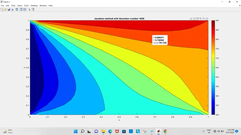
JACOBIAN METHOD

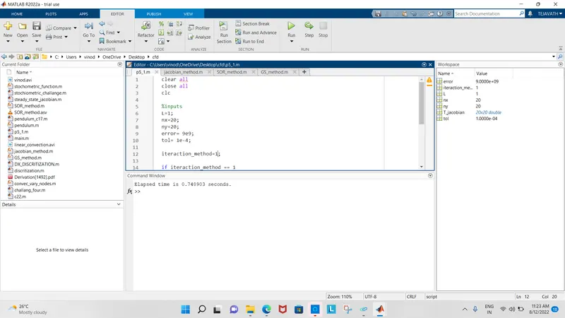
elapsed time

2. Gauss-siedel method

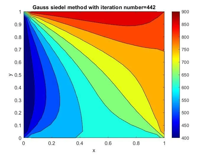
elapsed time is

3. Successive over relaxed method

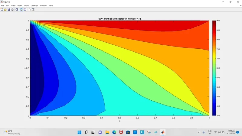
elapsed time: is 11.9098 seconds

observation:

As you can see from the above results Jacobi method has the highest number of iterations. Gauss-Siedel method has less number of iterations than the Jacobi method. Also, it can be seen that the SOR method is most efficient since it has less number of iterations and the elapsed time is very less. The SOR method really depends on the relaxation factor which I used here as omega (w). When we use the values more or less of 1.7 for omega calculated value will be away from the actual value, so iteration gets increased. so the preferred values are 1.7 and values around it.

B) Transient state explicit method

Here the equation for 2D heat conduction will be:

∂T∂t=α(∂2T∂x2+∂2T∂y2)∂T∂t=α(∂2T∂x2+∂2T∂y2)

alpha is the thermal diffusivity

So for the explicit method, we use nth terms for finding (n+1)th term

hence the equation is deformed as

Tn+1p=Tnp+k1(TL+TR)n+k2(TT+TB)n1+2k1+2k2Tpn+1=Tpn+k1(TL+TR)n+k2(TT+TB)n1+2k1+2k2

where k1=αΔtΔx2k1=αΔtΔx2

k2=αΔtΔy2k2=αΔtΔy2

as we use previous time step values to find the current time step value it is easy to calculate so we just keep them inside the time loop and space loop, no convergence loop will be used

% Solving the transient state 2D heat conduction problem using explicit method over a square domain.

clear all 
close all
clc
tic
%intial Conditions
L=1;
nx=20;
ny=nx;
% TEMPERATURE matrix
x=linspace(0,L,nx);
y=linspace(0,L,ny);
dx=L/(nx-1);
dy=L/(ny-1);
% TEMPERATURE matrix
T= 300*ones(nx,ny);

T_L = 400;
T_R = 800;
T_T = 600;
T_B = 900;

T(:,1)=T_L;
T(:,end)=T_R;
T(1,:)=T_T;
T(end,:)=T_B;
%edge refining 

T(1,1) = (T_L+T_T)/2;
T(1,end) = (T_T+T_R)/2;
T(end,1) = (T_L+T_B)/2;
T(end,end) = (T_B+T_R)/2;
Tprev=T;
dt=1e-4;
t=0.15;
nt=t/dt;
alpha=1;
k1=alpha*(dt/dx^2);
k2=alpha*(dt/dy^2);
 
for k=1:nt
    for i=2:nx-1
    for j=2:ny-1
   
    T(i,j)=Tprev(i,j)*(1-2*k1-2*k2)+k1*(Tprev(i-1,j)+Tprev(i+1,j))+k2*(Tprev(i,j-1)+Tprev(i,j+1));
    end
    end
    Tprev=T;

end
       figure(1)
contourf(x,y,T);
% clabel(C,h)
colormap(jet)
colorbar;
time_of_simulation=toc;
title_text = sprintf('solving 2D transient state heat equation explicitly \n time of simulation=%0.3f',time_of_simulation);
title(title_text)
xlabel('X axis')
ylabel('Y axis')

RESULTS OBTAINED:

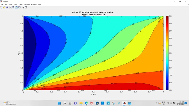
Explanation

Here we have the computation time as 231.216 seconds and our solution depends on CFL term

the CFL term here is

α(dtdx2+dtdy2)α(dtdx2+dtdy2)

we know that dx =dy

hence we can write it as

4α(Δt(Δx)2)4α(Δt(Δx)2)

the above term should be less than one, only then we can obtain the results correctly otherwise solution will blow up

C)Transient state implicit method

Instead of using nth term, we use n+1 th terms on the RHS

The equation formed for this will be

Tn+1p=Tnp+k1(TL+TR)n+1+k2(TT+TB)n+11+2k1+2k2Tpn+1=Tpn+k1(TL+TR)n+1+k2(TT+TB)n+11+2k1+2k2

Code for jacobian method

%function for jacobian method
function [jacobian_method]=steady_state_jacobian_implicit(L,nx,ny,error,tol)

tic

x = linspace(0,L,nx);
y = linspace(0,L,ny);
dx = L/(nx-1);
dy = L/(ny-1);
%Temperature matrix
T = 300*ones(nx,ny);
t = 0.14;
dt = 1e-4;
nt = t/dt;
Tleft = 400;
Tright = 800;
Ttop = 600;
Tbottom = 900;


T(:,1)= Tleft;
T(1,:) = Ttop;
T(:,end) = Tright ;
T(end,:) = Tbottom;
%defining the edge values
T(1,1) = (Ttop + Tleft)/2;
T(end,end) = (Tright+Tbottom)/2;
T(1,end) = (Ttop + Tright)/2;
T(end,1) = (Tbottom+Tleft)/2;
alpha =1;
k1 = alpha*(dt/dx^2);
k2 = alpha*(dt/dy^2);
Told = T;
Tpre = T;
j_iter = 1;

%convergance loop

while (error>tol)
    for i = 2:(nx-1)
        for j = 2:(ny-1)
            T(i,j) = (Tpre(i,j)+k1*(Told(i-1,j)+Told(i+1,j))+k2*(Told(i,j-1)+Told(i,j+1)))/(1+2*k1+2*k2);
        end
    end

    error = max(max(abs(Told-T)));
    Told = T;  %replacing the old value to new
    j_iter = j_iter + 1; %for continueing the itration process
    Tpre = T;
    %plotting
    figure(1)
    contourf(x,y,T)

    colormap(jet);
    colorbar %for showing color scale
    toc;
    pause (0.03)
    titletext = sprintf('jacobi method with iteration number=%d',j_iter);
    title(titletext);
    xlabel('x')
    ylabel('y')

end

end

2. Guass-siedel method

%function for GS method
function [Gauss_siedel]=steady_state_Gauss_siedel(L,nx,ny,error,tol)

tic

x = linspace(0,L,nx);
y = linspace(0,L,ny);
dx = L/(nx-1);
dy = L/(ny-1);
%Temperature matrix
T = 300*ones(nx,ny);
t = 0.14;
dt = 1e-4;
nt = t/dt;
Tleft = 400;
Tright = 800;
Ttop = 600;
Tbottom = 900;


T(:,1)= Tleft;
T(1,:) = Ttop;
T(:,end) = Tright ;
T(end,:) = Tbottom;
%defining the edge values
T(1,1) = (Ttop + Tleft)/2;
T(end,end) = (Tright+Tbottom)/2;
T(1,end) = (Ttop + Tright)/2;
T(end,1) = (Tbottom+Tleft)/2;
alpha = 1;
k1 = alpha*(dt/dx^2);
k2 = alpha*(dt/dy^2);
Told = T;
Tpre = T;
GS_iter = 1


while (error>tol)
    for i = 2:(nx-1);
    for j = 2:(ny-1) ;
        T(i,j) = (Tpre(i,j)+k1*(T(i-1,j)+Told(i+1,j))+k2*(T(i,j-1)+Told(i,j+1)))/(1+2*k1+2*k2);
    end
    end
    
    error = max(max(abs(Told-T)));
    Told = T;  %replacing the old value to new
    GS_iter = GS_iter + 1; %for continueing the itration process
    Tpre = T;
    %plotting
    figure(2)
    contourf(x,y,T) 
    
    colormap(jet);
    colorbar %for showing color scale
    toc;
    pause (0.03)
    titletext = sprintf('GS method with iteration number=%d',GS_iter);
    title(titletext);
    xlabel('x')
    ylabel('y')
   
end

end

3.SOR method

%function for sor method
function [SOR_method] =steady_state_sor(L,nx,ny,error,tol)

tic

x = linspace(0,L,nx);
y = linspace(0,L,ny);
dx = L/(nx-1);
dy = L/(ny-1);
%Temperature matrix
T = 300*ones(nx,ny);
t = 0.14;
dt = 1e-4;
nt = t/dt;
Tleft = 400;
Tright = 800;
Ttop = 600;
Tbottom = 900;


T(:,1)= Tleft;
T(1,:) = Ttop;
T(:,end) = Tright ;
T(end,:) = Tbottom;
%defining the edge values
T(1,1) = (Ttop + Tleft)/2;
T(end,end) = (Tright+Tbottom)/2;
T(1,end) = (Ttop + Tright)/2;
T(end,1) = (Tbottom+Tleft)/2;
alpha = 1;
w = 1.2;
k1 = alpha*(dt/dx^2);
k2 = alpha*(dt/dy^2);
Told = T;
Tpre = T;
SOR_iter = 1


while (error>tol)
    for i = 2:(nx-1);
    for j = 2:(ny-1) ;
        Tgs(i,j) = (Tpre(i,j)+k1*(T(i-1,j)+Told(i+1,j))+k2*(T(i,j-1)+Told(i,j+1)))/(1+2*k1+2*k2);
        T(i,j) = (1-w)*Told(i,j)+w*Tgs(i,j)
    end
    end
    
    error = max(max(abs(Told-T)));
    Told = T;  %replacing the old value to new
    SOR_iter = SOR_iter + 1; %for continueing the itration process
    Tpre = T;
    %plotting
    figure(3)
    contourf(x,y,T) 
    colormap(jet);
    colorbar %for showing color scale
    toc;
    pause (0.03)
    titletext = sprintf('SOR method with iteration number=%d',SOR_iter);
    title(titletext);
    xlabel('x')
    ylabel('y')
   
end

end

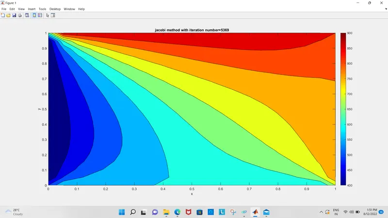
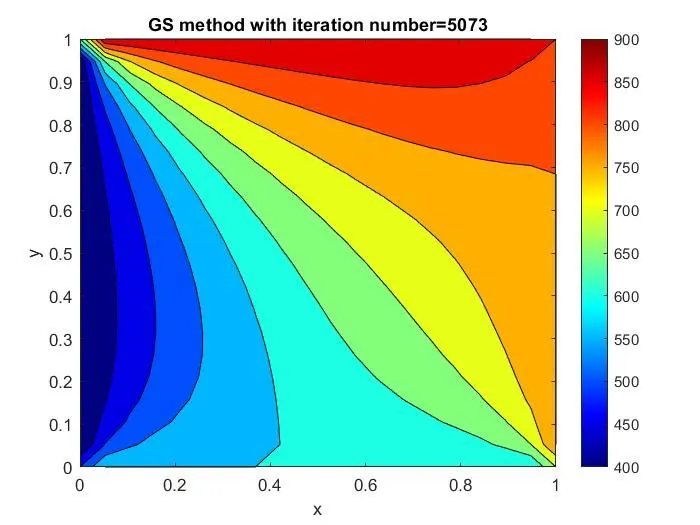
Results obtained

1. Jacobi Method

2. Guass-siedel method

elapsed time is 1577.87 seconds

3. SOR method

The elapsed time is 1903.73 seconds

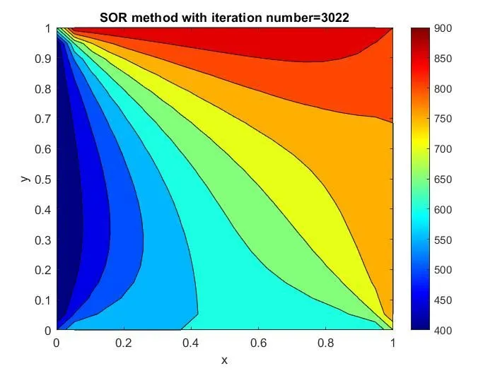
Explanation

Here we can see that the SOR method takes less time and less number of iterations, so the SOR method can be defined as an efficient method to solve transient heat equations implicitly. Jacobi method again comes up with a larger number of iterations and takes more time to calculate. We can also observe that the explicit method solves faster in time but for clarity of solution it depends upon the CFL term. While doing transient state SOR implicitly the solution depends on the value of omega (w). So the optimum value for omega came to be around 1.2.