Steady-State analysis & Transient-State Analysis in MATLAB by solving the 2-D heat conduction equation by using the Point Iterative Techniques.

Steady-state analysis & Transient State Analysis in MATLAB by solving the 2-D heat conduction equation by using the point iterative techniques.

AIM: To conduct Steady-state analysis & Transient State Analysis in MATLAB by solving the 2D heat conduction equation by using the point iterative techniques.

The Boundary conditions for the problem are as follows;

Top Boundary = 600 K

Bottom Boundary = 900 K

Left Boundary = 400 K

Right Boundary = 800 K

The following methods are to be used for solving implicit equations.

1. Jacobi

2. Gauss-seidel

3. Successive over-relaxation

The absolute error criteria is 1e-4.

THEORY:

Heat Conduction is the transfer of internal energy by microscopic collisions of particles and the movement of electrons within a body. The Heat Conduction is represented as a Partial Differential Equation that describes the distribution of heat in the given body over time. The 2-D Heat Conduction equation is represented as

The 2-D Unsteady-State Heat Conduction without heat generation(`q_v = 0`) withing the component is given by

`(delT)/(delt) + alpha((del^2T)/(delx^2) + (del^2T)/(dely^2)) = 0`

where `alpha` = Thermal Diffusivity.

The 2-D Steady-State(Time derivative is zero) Heat Conduction without heat generation(`q_v = 0`) within the component is given by

`(del^2T)/(delx^2) + (del^2T)/(dely^2) = 0`

where `alpha` = Thermal Diffusivity.

Discretization of Heat Conduction Equation

1. Unsteady-State 2-D Heat Conduction:

`(delT)/(delt) + alpha((del^2T)/(delx^2) + (del^2T)/(dely^2)) = 0`

For the Time Derivative term forward differencing is used as it is the Time Marching process and Central Differencing is used for the Space Derivative.

The Discretization process of the heat conduction equation is shown below

`(T_(i,j)^(n+1)-T_(i,j)^n)/(triangleT) = alpha((T_R-2T_P+T_L)/(trianglex^2) + (T_T-2T_P+T_B)/(triangley^2))^n`

`T_(i,j)^(n+1)=T_(i,j)^n+alphatriangleT((T_R-2T_P+T_L)/(trianglex^2) + (T_T-2T_P+T_B)/(triangley^2))^n`

`T_(i,j)^(n+1)=T_(i,j)^n+k_1(T_R-2T_P+T_L)^n + k_2(T_T-2T_P+T_B)^n`

where n = Time step, i,j = position,

T_R = T(i+1,j) at time step n

T_L = T(i-1,j) at time step n

T_T = T(i,j+1) at time step n

T_B = T(i,j-1) at time step n

T_P = T(i,j) at time step n

2. Steady-State 2-D Heat Conduction:

`(del^2T)/(delx^2) + (del^2T)/(dely^2) = 0`

For the Time Derivative term forward differencing is used as it is the Time Marching process and Central Differencing is used for the Space Derivative.

The Discretization process of the heat conduction equation is shown below

`(T_R-2T_P+T_L)/(trianglex^2) + (T_T-2T_P+T_B)/(triangley^2) = 0`

`2T_P(1/(trianglex^2)+1/(triangley^2))=(T_R+T_L)/(trianglex^2) + (T_T+T_B)/(triangley^2)`

`T_P = 1/k((T_R+T_L)/(trianglex^2) + (T_T+T_B)/(triangley^2))`

where

`k = 2(trianglex^2+triangley^2)/(trianglex^2*triangley^2`

T_R = T(i+1,j) at time step n

T_L = T(i-1,j) at time step n

T_T = T(i,j+1) at time step n

T_B = T(i,j-1) at time step n

T_P = T(i,j) at time step n

Method of Solving the Partial derivatives

1. Explicit Method

In the Explicit approach, each difference equation has only one unknown and therefore it is solved explicitly for this unknown in a straightforward manner. The Explicit approach for solving the Unsteady-State 2-D Heat Conduction is shown below

`T_(i,j)^(n+1)=T_(i,j)^n+k_1(T_R-2T_P+T_L)^n + k_2(T_T-2T_P+T_B)^n`

In the above equation, the temperature at node(i,j) at time step n+1 is calculated using the temperature at different nodes from the previous time step.

2. Implicit Method

In the Implicit approach, the unknowns are obtained from the simultaneous solution of the difference equation applied at all the grid points arrayed at a single timestep.

The Implicit approach for solving the Unsteady-State 2-D Heat Conduction is shown below

`T_(i,j)^(n+1)=T_(i,j)^n+k_1(T_R-2T_P+T_L)^(n+1) + k_2(T_T-2T_P+T_B)^(n+1)`

To solve this problem the Iterative Method is used. Iterative Method is a method of solving this kind of problems in which the unknown values given with random values and updating the values after each iteration so that the solution converges to a single value.

There are three Iterative Methods and they are

1. Jacobi Method

2. Gauss-Seidel Method

3. Successive over Regression method.

Jacobi Method

In numerical linear algebra, the Jacobi method is an iterative algorithm for determining the solutions of a strictly diagonally dominant system of linear equations. Each diagonal element is solved for, and an approximate value is plugged in. The process is then iterated until it converges. The Jacobi method for solving the Unsteady-State 2-D Heat Conduction is shown below

`T_(i,j)^(k+1)=1/(1+2k_1+k_2)(T_(i,j)^k+k_1(T_R^k+T_L^(k)) + k_2(T_T^k+T_B^(k)))`

Where, k = iteration number.

The Jacobi method for solving the Steady-State 2-D Heat Conduction is shown below

`T_P^(k+1) = 1/k_t((T_R^k+T_L^(k))/(trianglex^2) + (T_T^k+T_B^(k))/(triangley^2))`

Gauss-Seidel Method

In numerical linear algebra, the Gauss-Seidel method is an iterative method used to solve a system of linear equations. Each diagonal element is solved for, and an approximate value is plugged in. This process is then iterated until it converges and during each iteration, the solved values are updated simultaneously and the updated values are used to solve the next unknown in the same iteration.

The Gauss-Seidel method for solving the Unsteady-State 2-D Heat Conduction is shown below

`T_(i,j)^(k+1)=1/(1+2k_1+k_2)(T_(i,j)^k+k_1(T_R^k+T_L^(k+1)) + k_2(T_T^k+T_B^(k+1)))`

Where, k = iteration number.

The Gauss-Seidel method for solving the Steady-State 2-D Heat Conduction is shown below

`T_P^(k+1) = 1/k_t((T_R^k+T_L^(k+1))/(trianglex^2) + (T_T^k+T_B^(k+1))/(triangley^2))`

Successive Over Regression Method(SOR)

Succession over Regression method is a variant of the Gauss-Seidel Method. In this method, the solution is updated adding the slope of the variation of result and multiplying with the scaling factor to the output from each iteration. The SOR method for solving the Unsteady-State 2-D Heat Conduction is shown below

`T^(k+1) = T^k+omega(T^(k+1)-T^(k))/(k+1-k)`

`implies``T^(k+1) =(1-omega) T^k+omegaT^(k+1)`

where `T^(k+1)` in the right-hand side is already calculated using Gauss-Seidel Method and the result is again updated using this method.

PROCEDURE:

1. Unsteady-State 2-D Heat Conduction using Implicit Method(Jacobi Method)

The program developed uses the same equations derived for different methods for solving 2-D Heat Conduction. The flow of the program is shown below

1. Clearing the workspace and command window and closing all the figures opened.
2. Defining Boundary condition.
3. Defining the parameters required for the problem.
4. Creating Temperature Matrix.
5. Solving the Heat Conduction Equation.
6. Plotting the variation of the result in each iteration.

Step 1: Clearing the workspace and command window and closing all the figures opened.

Clear all command clears the workspace, close all command closes the figures opened and clc command clears the command window. Below syntax is used to do the same.

clear all
close all
clc

Step 2: Defining Boundary condition.

In this program, the boundary condition is Temperature at the boundary of the domain.

Below syntax is used to define the boundary condition.

% Boundary Condition
T_L = 400;              % Left End Temperature
T_R = 800;              % Right End Temperature
T_T = 600;              % Top End Temperature
T_B = 900;              % Botttom End Temperature

Step 3: Defining the parameters required for the calculation

Below syntax is used to define the parameters that are required in solving the problem

% Parameters for the program 
n = 11;                 % Number of nodes
x = linspace(0,1,n);    % x_axis
dx = x(1)-x(2);         % dx

y = x;                  % y = x
dy = dx;                % dy = dx

q = 1;

[xx yy] = meshgrid(x,y);

error = 1e10;           % Error defined as initial condition    
tolerence = 1e-4;       % Tolerence for the result

dt = 1e-2;              % Time Step

alpha = 0.25;

% For Unsteady-State heat condution

k_1 = alpha*dt/(dx^2); % Simplifiying the equation
k_2 = alpha*dt/(dy^2);

In the above syntax, k1 and k2 are the Courants number and the sum of those two number should always be less than 0.5.

Step 4: Creating a Temperature Matrix.

In this temperature matrix, all the inside value are assumed except the boundary values. Below syntax is used to create the temperature matrix.

% Temperature Matrix
T = 300*ones(n,n);

T(:,1) = T_L;
T(1,:) = T_T;
T(:,end) = T_R;
T(end,:) = T_B;

T(1,1) = (T_L + T_T)/2;
T(1,end) = (T_T + T_R)/2;
T(end,1) = (T_B + T_L)/2;
T(end,end) = (T_R + T_B)/2;
T_old = T;              % Upadating the old value intially

At the end of the syntax, T_old is created and the matrix T values are made to store in T_old. This matrix is used further in the iteration method.

Step 5: Solving the Heat Conduction Equation

While solving the 2-D Heat condition using the Implicit method two for loop is used for storing the values for all the points in the matrix and a while loop is used to run the iteration until the error is less than the tolerance values given.

Below syntax is used to solve the 2-D Unsteady-State Heat Conduction using Jacobi Method.

for t = 1:nt                            % Time loop
error = 9e9;                            % Updating error for each Time Step
while error > tolerance                 % Loop will run until the error is less than tolerance value
        % Space Loop
        for i = 2:n-1                       % x -  Coordinate
            
            for j = 2:n-1                   % y -  Coordinate
                
                T(i,j) = (k_1*(T_old(i-1,j) + T_old(i+1,j)) + k_2*(T_old(i,j+1) + T_old(i,j-1)) + T_old(i,j))*term_1;
                
            end
            
        end
        error = max(max(abs(T_old - T)));  % Finding the error
        T_old = T;                         % Updating the Temperature
 
end       
%Plotting 
...

end

In the above syntax, the error is calculated by finding the absolute maximum of the difference between the current and last iteration values and the T_old is updated once all the values are calculated for all the points in the matrix.

Step 6: Plotting the variation of the result after each time step.

For this temperature matrix, a contour plot is done to see the variation of the values during each iteration. Below syntax is used inside the time loop so as to display the result for each time step.

contourf(xx,yy,T)
title_01 = sprintf('Number of Iteration = %d',q);
title(title_01)
colormap hot 
pause(0.01)
q = q + 1;            % Iteration Counter

2. Steady-State 2-D Heat Conduction using Implicit Method using Jacobi Iteration Method.

The Program for the Steady-State 2-D Heat Conduction is almost the same as the unsteady state heat conduction but the only change is that the time loop is not there and the Equation to find the Temperature at a particular grid point is different. The Syntax used in calculating the Temperature is shown below

term_1 = 2*(dx^2+dy^2)/(dx*dy)^2;           % Simplifying the Equation  
    while error > tolerance                 % Loop will run untill the error is less than tolerance value
        
        for i = 2:n-1                       % x -  Coordinate
            
            for j = 2:n-1                   % y -  Coordinate
                
                T(i,j) = ( ((T_old(i+1,j) + T_old(i-1,j)) / dx^2)  +  (( T_old(i,j+1) + T_old(i,j-1) ) / dy^2) )/term_1;
                
            end
            
        end
        

        error = max(max(abs(T_old - T)));  % Finding the error
        T_old = T;                         % Updating the Temperature
        
        contourf(xx,yy,T)                  % Plotting Temperature Domain 2-D 
        title_01 = sprintf('Number of Iteration = %d',q);
        title(title_01)
        colormap hot 
        colorbar
        pause(0.001)
        
        q = q + 1;                         % Iteration Counter
    end
  

3. Unsteady-State 2-D Heat Conduction using Explicit Method.

The program for Explicit method for solving the Unsteady State Heat Conduction is almost same as the Implicit method but the calculation part in the program is different. The Calculation of Temperature at next time step using explicit method is shown below.

for e = 1:nt                        % Time Loop
        
     for i = 2:n-1                  % Space Loop x

          for j = 2:n-1             % Space Loop y
              
                % Calculation of temperature using Explicit Method
                T(i,j) = T_old(i,j) + k*(((T_old(i+1,j)-2*T_old(i,j)+T_old(i-1,j))/dx^2)+((T_old(i,j+1)-2*T_old(i,j)+T_old(i,j-1))/dy^2));
                

          end
     end
     
    % Time Step Counter 
    q = q+1;
    
    % Plotting
    contourf(xx,yy,T)
    title(q)
    colormap hot 
    pause(0.01)
    
    T_old = T;                      % Updating the Temperature 
end

4. Steady-State 2-D Heat Conduction using Implicit Method with Gauss-Seidel Iteration Method.

The program for Implicit method for solving the Steady State Heat Conduction using Gauss-Seidel Iteration method is almost same as the Jacobi Method but the calculated values are updated for each point. The Calculation of Temperature at next time step using explicit method is shown below.

 % Calculation of Temperature using Gauss-Seidel Method
T(i,j) = ( ((T_old(i+1,j) + T(i-1,j)) / dx^2)  +  (( T_old(i,j+1) + T(i,j-1) ) / dy^2) )/term_1;

In the above syntax the Temperature at (i+1,j+1) node is calculated using the updated value at (i,j) node.

5. Unsteady-State 2-D Heat Conduction using Implicit Method with SOR Iteration Method.

The program for Implicit method for solving the Steady State Heat Conduction using SOR Iteration method is a variant of Gauss-Seidel Method. The Calculation of Temperature at next time step using explicit method is shown below.

 % Calculation of Temperature using Gauss-Seidel Method
 T(i,j) = ( ((T_old(i+1,j) + T(i-1,j)) / dx^2)  +  (( T_old(i,j+1) + T(i,j-1) ) / dy^2) )/term_1;
% Calculation of Temperature using SOR method
T(i,j) = (1-w)*T_old(i,j) + w*T(i,j);
                

In the above syntax, fi the temperature is calculated using Gauss-seidel Method and it is updated using the SOR formula as mentioned earlier.

6. Unsteady-State 2-D Heat Conduction using Implicit Method with Gauss-Seidel Iteration Method.

The program for Implicit method for solving the Unsteady State Heat Conduction using Gauss-Seidel Iteration method is almost same as the Jacobi Method but the calculated values are updated for each point. The Calculation of Temperature at next time step using explicit method is shown below.

% Calculation of Temperature using Gauss-Seidel Method
T(i,j) = (k_1*(T(i-1,j) + T_old(i+1,j)) + k_2*(T_old(i,j+1) + T(i,j-1)) + T_P(i,j))*term_1;

In the above syntax the Temperature at (i+1,j+1) node is calculated using the updated value at (i,j) node.

7. Unsteady-State 2-D Heat Conduction using Implicit Method with SOR Iteration Method.

The program for Implicit method for solving the Unsteady State Heat Conduction using SOR Iteration method is a variant of Gauss-Seidel Method. The Calculation of Temperature at next time step using explicit method is shown below.

% Calculation of Temperature using Gauss-Seidel Method
T(i,j) = (k_1*(T(i-1,j) + T_old(i+1,j)) + k_2*(T_old(i,j+1) + T(i,j-1)) + T_old(i,j))*term_1;
% Calculation of Temperature using SOR method
T(i,j) = (1-w)*T_old(i,j) + w*T(i,j);
                

In the above syntax first the temperature is calculated using Gauss-seidel Method and it is updated using the SOR formula as mentioned earlier.

COMPLETE PROGRAM:

1. Steady-State 2-D Heat Conduction(Implcit Method-Jacobi method)

clear all
close all
clc

% Parameters for the program 
n = 11;                 % Number of nodes
x = linspace(0,1,n);    % x_axis
dx = x(1)-x(2);         % dx

y = x;                  % y = x
dy = dx;                % dy = dx

q = 1;

[xx yy] = meshgrid(x,y);

error = 1e10;           % Error defined as initial condition    
tolerance = 1e-4;       % Tolerence for the result

dt = 1e-2;
n_t = 40;


% Boundary Condition
T_L = 400;              % Left End Temperature
T_R = 800;              % Right End Temperature
T_T = 600;              % Top End Temperature
T_B = 900;              % Botttom End Temperature

% Temperature Matrix
T = 300*ones(n,n);

T(:,1) = T_L;
T(1,:) = T_T;
T(:,end) = T_R;
T(end,:) = T_B;

T(1,1) = (T_L + T_T)/2;
T(1,end) = (T_T + T_R)/2;
T(end,1) = (T_B + T_L)/2;
T(end,end) = (T_R + T_B)/2;

T_old = T;              % Upadating the old value intially

% Jacobi Iteration Method of Solving the PDE

term_1 = 2*(dx^2+dy^2)/(dx*dy)^2;           % Simplifying the Equation


    
    while error > tolerance                 % Loop will run untill the error is less than tolerence value
        
        for i = 2:n-1                       % x -  Coordinate
            
            for j = 2:n-1                   % y -  Coordinate
                
                T(i,j) = ( ((T_old(i+1,j) + T_old(i-1,j)) / dx^2)  +  (( T_old(i,j+1) + T_old(i,j-1) ) / dy^2) )/term_1;
                
            end
            
        end
        

        error = max(max(abs(T_old - T)));  % Finding the error
        T_old = T;                         % Updating the Temperature
        
        contourf(xx,yy,T)                  % Plotting Temperature Domain 2-D 
        title_01 = sprintf('Number of Iteration = %d',q);
        title(title_01)
        colormap hot 
        colorbar
        pause(0.001)
        
        q = q + 1;                         % Iteration Counter
    end

2. Unsteady-State 2-D Heat Conduction(Implicit Method-Jacobi Method)

clear all
close all
clc

% Parameters for the program 
n = 11;                 % Number of nodes
x = linspace(0,1,n);    % x_axis
dx = x(1)-x(2);         % dx

y = x;                  % y = x
dy = dx;                % dy = dx

q = 1;

[xx yy] = meshgrid(x,y);

error = 1e10;           % Error defined as initial condition    
tolerence = 1e-4;       % Tolerence for the result

dt = 1e-2;              % Time Step
nt = 200;               % Number of Time steps  

alpha = 0.25;

k_1 = alpha*dt/(dx^2); % Simplifiying the equation
k_2 = alpha*dt/(dy^2);


% Boundary Condition
T_L = 400;              % Left End Temperature
T_R = 800;              % Right End Temperature
T_T = 600;              % Top End Temperature
T_B = 900;              % Botttom End Temperature

% Temperature Matrix
T = 300*ones(n,n);

T(:,1) = T_L;
T(1,:) = T_T;
T(:,end) = T_R;
T(end,:) = T_B;

T(1,1) = (T_L + T_T)/2;
T(1,end) = (T_T + T_R)/2;
T(end,1) = (T_B + T_L)/2;
T(end,end) = (T_R + T_B)/2;

T_old = T;
T_P = T;
% Jacobi Iteration Method of Solving the PDE

term_1 = 1/(1+2*(k_1+k_2));

tic
for t = 1:nt                        % Time Loop
    error  = 9e9;                   % Updating the error
    d = 1;
    while error > tolerence 
        
        for i = 2:n-1               % Space loop x
            
            for j = 2:n-1           % Space Loop y
                % Calculation of Temperature using Jacobi Method
                T(i,j) = (k_1*(T_old(i-1,j) + T_old(i+1,j)) + k_2*(T_old(i,j+1) + T_old(i,j-1)) + T_P(i,j))*term_1;
                
            end
            
        end  
        
        d = d+1;
        
        % Calculation of error 
        error = max(max(abs(T_old - T)));
        T_old = T;                  % Updating the old iteration value of Temperature
        

    end
    T_P = T;
    % Plotting the Temperature
    
        
    contourf(xx,yy,T)
    title_01 = sprintf('Number of Time Step = %d',q);
    title(title_01)
    colormap hot 
    pause(0.01)
    q = q + 1;  % Time Step Counter

end

toc

The rest of the 5 programs is attached below.

RESULTS:

1. Steady-State 2-D Heat Conduction

The Steady-State analysis can only be done by the Implicit method as there are more than one unknowns in the equation. The below table shows the number of iterations done to arrive at a solution.

Iteration Methods	Number of Iterations to arrive at Solution
Jacobi iteration Method	252
Gauss-Seidel Method	135
SOR Method	39

The number of iterations to arrive at solution for Gauss-Seidel method is nearly half of the Jacobi Method and the and in case of SOR method it is nearly 1/3rd as that of Gauss-Seidel method. The number of iteration in the Gauss-Seidel is less than that of the Jacobi method as the temperature is updated after the calculation of each point in the temperature matrix. And in the SOR method it is Number of iteration to arrive at the solution depends on the scaling factor used. For scaling factor `omega = 1.5` the number of iterations is 39. The below image shows the contour plot of the temperature matrix at the last iteration in the Jacobi method.

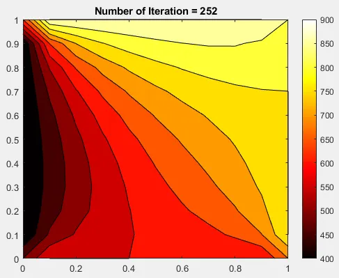
Image 1. Contour Plot of Temperature Matrix

2. Unsteady-State 2-D Heat Conduction

The Unsteady-State 2-D Heat Conduction can be done in two methods Implicit and Explicit methods as there can be only one unknown for the Explicit method and can have more than one unknown for Implicit method.

Implicit Method

In the implicit method, the run time for the Gauss-Seidel and SOR method was nearly twice of the Jacobi Method for the same number of time step.

Iteration Methods	Run Time
Jacobi iteration Method	14.19 sec
Gauss-Seidel Method	29.18 sec
SOR Method	29.52 sec

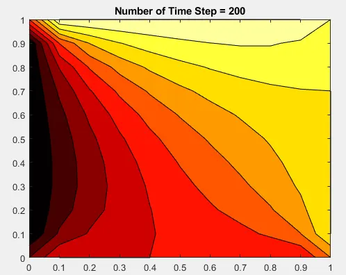
Image 2. Contour Plot of the Temperature matrix at the last time step.

CONCLUSION:

7 Programs were created for each and every type of analysis and all 7 programs ran without errors. In each program contour plot of temperature matrix for each iteration for steady-state analysis and contour plot for each time step in Unsteady State analysis.

Implicit vs Explicit Analysis

Implicit Analysis is used when the matrix inversion is very difficult i.e if there are many number of nodes or grid points and inverting those matrices will be very difficult. On applying this method i.e by solving the unknowns simultaneously from the iteration method, the solution is obtained in a faster way. This method is unconditionally stable and facilitate larger time steps. Despite this advantage, the implicit methods can be extremely time-consuming when solving dynamic and nonlinear problems.

The Explicit analysis is used where the matrix is small and the inversion of it is easy(less time consuming). In many cases, the matrix is lumped and thus diagonal matrix. Inversion of those matrices is straightforward and includes the only inversion of only diagonal terms. In these calculations, the scheme is not unconditionally stable and thus smaller time steps are required. The solution in the explicit method depends on the Courant Number and it should be less than 0.5 for stable output.