Week 5.1 - Mid term project - Solving the steady and unsteady 2D heat conduction problem

Aim :

Solve the 2D heat conduction equation by using the point iterative techniques and explicit iterative techniques.

CODE & EXPLANATION :

Here we are going to understand the concept of the 2d heat conduction equation of both stead and transient state of flow. We need to understand the derivation part where the terms are being discretized sequentially and then we move on to the coding part. There are few things that need to be considered before going over it is that for steady-state we need to apply iterative solvers and for transient, we have to solve both the schemes we seen in the previous section as IMPLICIT and EXPLICIT.

Now we are going to understand the derivation part of the steady-state condition.

Solving this by

1. Jacobi

2. Gauss-seidel

3. Successive Over Relaxation SOR

since `(d^2*t)/dx^2 +(d^2*t)/dy^2 = 0`, its has elliptic nature properties which we an discretize them using central differencing scheme

clear all
close all
clc

% EXPLICIT 2D HEAT CONDUCTION UNSTEADY STATE PROBLEM.
nx = 50;
ny = 40;
nt = 1800;
dt = 1e-5;
L = 1; % Length of X
W = 1; % Length of Y
dx = L / (nx-1); % Grid point length
dy = W / (ny-1); % Grid point length
T = 300*ones(50,40);
TL = 400;
TT = 600;
TB = 900;
TR = 800;
T(1,:) = TT;
T(end,:) = TB;
T(:,1) = TL;
T(:,end) = TR;
T(1,1) = (TT+TL)*0.5;
T(end,1) = (TL+TB)*0.5;
T(1,end) = (TR+TT)*0.5;
T(end,end) = (TR+TB)*0.5;
alpha = 1.4;

% CFL 1
k1 = alpha * (dt / dx^2)
% CFL 2 
k2 = alpha * (dt / dy^2)

T_initial = T;
Told = T;
T_calc = T;
iter = 0;
error = 1;
tol = 1e-4;
tic;
for g = 1 : nt
    while (error > tol)
        for i = 2 : (nx-1)
            for j = 2 : (ny-1)
     
                T_L = Told(i-1,j) ; T_R = Told(i+1,j) ; T_T = Told(i,j+1) ; T_B = Told(i,j-1);
                Term_1 = Told(i,j) ; Term_2 = k1 * (T_R - 2 * Term_1 + T_L) ; Term_3 = k2 * (T_T - 2 * Term_1 + T_B);
                T_calc(i,j) =  Term_1 + Term_2 + Term_3;
        
            end
            iter = iter + 1;
            error(iter) = max(max(abs(T_calc - Told)));
            Told = T_calc;
        end
    end
end
t1 = toc;
figure(1)
contourf(flipud(T_calc),'ShowText','ON')
colormap(jet)
xlabel('X-Axis')
ylabel('Y-Axis')
title(sprintf('No. of Iterations = %d Simulation Time = %fs dt = %d',iter,t1,dt));
            
            
            

Heat conduction equation is define by the pde,

which is the heat distribution in 3D space with the period of time.

where alpha is known to be '\ thermal diffusivity \' (m^2/s)

Given that, the number of grid points in x direction is equal to y direction and the domain is assumed to be an unit square.

Boundary conditions given,

1. Left (TL) = 400K 2. Right (TR) = 800K 3. Top(TT) = 600K 4. Bottom (TB) = 900K

First let's define what are the iterative techniques we are using here:

1. Jacobi

In this iteration technique we assume the initial values at all nodes to calculate the new values, which will updated once we find the all the nodes values and this process will goes on untill we arrive with an converge solution. For different simulateneous equations with many unknowns first we have to make the equations into Diagonally dominant matrix form for converging results.

2. Gauss-seidel

In this iteration we assume the values obtained in Jacobi iteration for the next equation immediately without waiting for completion of first cycle.

3. Successive Over-relaxation (SOR)

This method is an updated version of previous two. In addition we use the relaxation factor to ease the process. For this analysis we use the relaxation facor to be greater than 1 and less than 2.

Explanation of the Main Script:

1. Specifying the number of grid points in the spacial domain x and y direction. In this case is 10 grid points in x and y direction.

2. Specifying the length of the domain in x and y space domain.

3. Defining the spacial domain for the length and grid points specified.

4. Calculating the grid spacing in the x and y space domain.

5. Defining temperature with the guess values 300K for the number of the grid points defined.

6. Applying the Boundary Conditions as mentioned in the problem.

7. The accuracy of the solution is measured with computed approximated solution and compared with the tolerance value so that the converged solution is in the desired accuracy.

8. A copy of the initial temperature matrix is made in told and t_pre which is used while calculating the temperature values of n+1 time steps explicitly and implicitly.

9. Calculating all the K's. Here alpha is taken 1.4.

10. Function is called to calculate the temperature values at n+1 time step for both steady and unsteady state using different iterative solvers and explicit method is also used for calculating temperature for unsteady state heat conduction equation.

Explanation of Functions defined in the main script:

In the functions dummy error is assigned to error variable so that the while loop condition would satisfy and iterations are calculated.

The error is calculated and updated for each iteration. The error calculated is coded to take only the absolute values since negative values will not statisfy the while loop condition and iterations will stopped and the results obtained will not be a converged results.

Number of iterations taken for the solution to converge is stored in the iter variable. This is done by increamenting the iter variable by 1 for each iteration.

As the iteration proceeds to calculate temperature at n+1 time step temperature at nth time step is required and these temperature values should be updated for each iteration. If the temperature values are not updated for each iteration the solution will not converge and while loop will run infinite times.

Contourf plot is used to check if the solutions are converged or not i.e., the plot does not change as the approximated temperature value changes in the order of tolerance value defined.

told stores the temperature values of the preceeding time step.

t stores the temperature values of the n+1 time step.

This logic is used in the below functions to calculate the temperature of Steady state Heat Conduction equation for the desired accuracy.

%Jacobi Iteration

close all
clear all
clc

%Solving the Unsteady state 2D heat conduction by Jacobi Method(IMPLICIT SCHEME)

%Input Parameters
nx = 10;
ny = nx;
nt = 1600;

x = linspace(0,1,nx);
y = linspace(0,1,ny);

dx = x(2) - x(1);
dy = dx;


%Absolute error criteria > tolerance
error = 1e9;
tolerance = 1e-4;
dt=1e-3

%Defining Boundary conditions
T_L = 400;
T_T = 600;
T_R = 800;
T_B = 900;

T = 300*ones(nx,ny);

T(2:ny - 1, 1)  = T_L;
T(2:ny - 1, nx) = T_R;
T(1, 2:nx - 1)  = T_T;
T(ny, 2:nx - 1) = T_B;

%Calculating Average temperature at corners
T(1,1) = (T_T + T_L)/2;
T(nx,ny) = (T_R + T_B)/2;
T(1,ny) = (T_T + T_R)/2;
T(nx,1) = (T_L + T_B)/2;

%Assigning orginal values to T
T_old = T;
T_intial = T;

%Calculation of 2D steady heat conduction EQUATION by Successive over-relaxation method
k1 = 1.1*(dt/(dx^2));
k2 = 1.1*(dt/(dy^2));

Jacobi_iteration = 1;
for k = 1:nt
    error = 1e9; 
    while(error > tolerance)
        
        for i = 2:nx - 1
            
            for j = 2:ny - 1
                    
                Term_1 = 1/(1 + (2*k1) + (2*k2));
                Term_2 = k1*Term_1;
                Term_3 = k2*Term_1;
                H = (T_old(i-1,j)) + (T_old(i+1,j));
                V = (T_old(i,j+1)) + (T_old(i,j-1));
                    
                T(i,j) = (T_intial(i,j)*Term_1) + (H*Term_2) + (V*Term_3);
   
            end
            
        end
        
        error = max(max(abs(T_old - T)));
        T_old = T;
        Jacobi_iteration = Jacobi_iteration + 1;  
        
    end
    T_intial = T;
end
%Plotting
figure
contourf(flipud(T),'ShowText','ON')
colorbar
xlabel('X-Axis')
ylabel('Y-Axis')
title(sprintf('No. of Jacobi Iterations = %d', Jacobi_iteration));

%Gauss-Siedel Iteration

close all
clear all
clc

%Solving the Unsteady state 2D heat conduction by Gauss Seidel Method(IMPLICIT SCHEME)

%Input Parameters
%Number of grid points
nx = 10;
ny = nx;
nt = 1600;

x = linspace(0,1,nx);
y = linspace(0,1,ny);

dx = x(2) - x(1);
dy = dx;

%Absolute error criteria > tolerance
error = 1e9;
tolerance = 1e-4;
dt = 1e-3;

%Defining Boundary conditions
T_L = 400;
T_T = 600;
T_R = 800;
T_B = 900;

T = 300*ones(nx,ny);

T(2:ny - 1, 1)  = T_L;
T(2:ny - 1, nx) = T_R;
T(1, 2:nx - 1)  = T_T;
T(ny, 2:nx - 1) = T_B;

%Calculating Average temperature at corners
T(1,1) = (T_T + T_L)/2;
T(nx,ny) = (T_R + T_B)/2;
T(1,ny) = (T_T + T_R)/2;
T(nx,1) = (T_L + T_B)/2;

%Assigning orginal values to T
T_old = T;
T_intial = T;

%Calculation of 2D steady heat conduction EQUATION by Successive over-relaxation method
k1 = 1.1*(dt/(dx^2));
k2 = 1.1*(dt/(dy^2));

Gauss_Seidel_iteration = 1;
for k = 1:nt
    error = 1e9; 
    
    while(error > tolerance)
        
        for i = 2:nx - 1
            
            for j = 2:ny - 1
                    
                Term_1 = 1/(1 + (2*k1) + (2*k2));
                Term_2 = k1*Term_1;
                Term_3 = k2*Term_1;
                H = (T(i-1,j)) + (T_old(i+1,j));
                V = (T(i,j+1)) + (T_old(i,j-1));
                    
                T(i,j) = (T_intial(i,j)*Term_1) + (H*Term_2) + (V*Term_3);
   
            end
            
        end
        
        error = max(max(abs(T_old - T)));
        T_old = T;
        Gauss_Seidel_iteration = Gauss_Seidel_iteration + 1;  
        
    end
    T_intial = T;
    
end
%Plotting
figure
contourf(flipud(T),'ShowText','ON')
colorbar
xlabel('X-Axis')
ylabel('Y-Axis')
title(sprintf('No. of Gauss Seidel iteration = %d', Gauss_Seidel_iteration));

%Successive over-relaxation

close all
clear all
clc

%Solving the Unsteady state 2D heat conduction by Successive over-relaxation Method(IMPLICIT SCHEME)

%Input Parameters
%Number of grid points
nx = 10;
ny = nx;
nt = 1600;

x = linspace(0,1,nx);
y = linspace(0,1,ny);

dx = x(2) - x(1);
dy = dx;

%Absolute error criteria > tolerance
error = 1e9;
tolerance = 1e-4;
dt = 1e-3;
omega = 1.1;

%Defining Boundary conditions
T_L = 400;
T_T = 600;
T_R = 800;
T_B = 900;

T = 300*ones(nx,ny);

T(2:ny - 1, 1)  = T_L;
T(2:ny - 1, nx) = T_R;
T(1, 2:nx - 1)  = T_T;
T(ny, 2:nx - 1) = T_B;

%Calculating Average temperature at corners
T(1,1) = (T_T + T_L)/2;
T(nx,ny) = (T_R + T_B)/2;
T(1,ny) = (T_T + T_R)/2;
T(nx,1) = (T_L + T_B)/2;

%Assigning orginal values to T
T_old = T;
T_intial = T;
T_end = T;

%Calculation of 2D steady heat conduction EQUATION by Successive over-relaxation method
k1 = 1.1*(dt/(dx^2));
k2 = 1.1*(dt/(dy^2));

Successive_over_relaxation_iteration = 1;
for k = 1:nt
    error = 1e9; 
    
    while(error > tolerance)
        
        for i = 2:nx - 1
            
            for j = 2:ny - 1
                    
                Term_1 = 1/(1 + (2*k1) + (2*k2));
                Term_2 = k1*Term_1;
                Term_3 = k2*Term_1;
                H = (T(i-1,j)) + (T_old(i+1,j));
                V = (T(i,j+1)) + (T_old(i,j-1));
                    
                T(i,j) = (T_intial(i,j)*Term_1) + (H*Term_2) + (V*Term_3);
                T_end(i,j) = ((1-omega)*T_old(i,j)) + (T(i,j)*omega);
                
            end
            
        end
        
        error = max(max(abs(T_old - T)));
        T_old = T_end;
        Successive_over_relaxation_iteration = Successive_over_relaxation_iteration + 1;  
        
    end
    
    T_intial = T_end;
    
end
%Plotting
figure
contourf(flipud(T),'ShowText','ON')
colorbar
xlabel('X-Axis')
ylabel('Y-Axis')
title(sprintf('No. of Successive-over relaxation iteration = %d',  Successive_over_relaxation_iteration));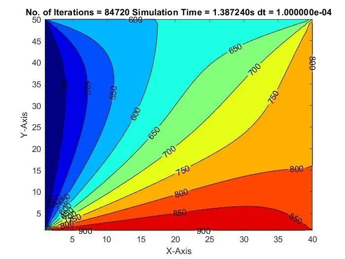

Inference from the Plots:

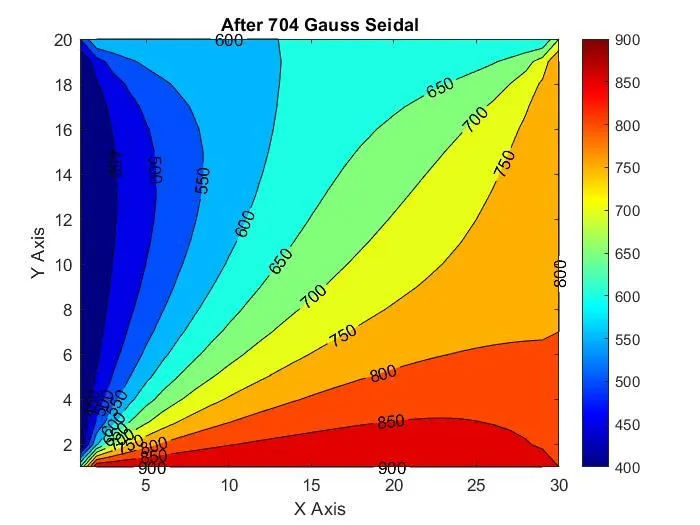
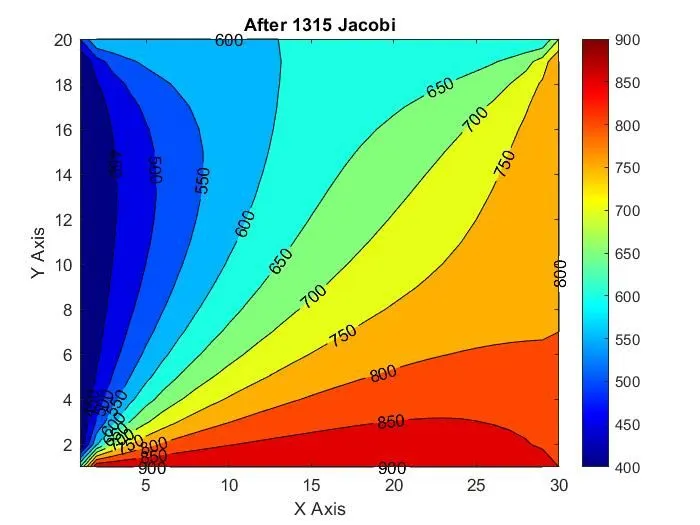
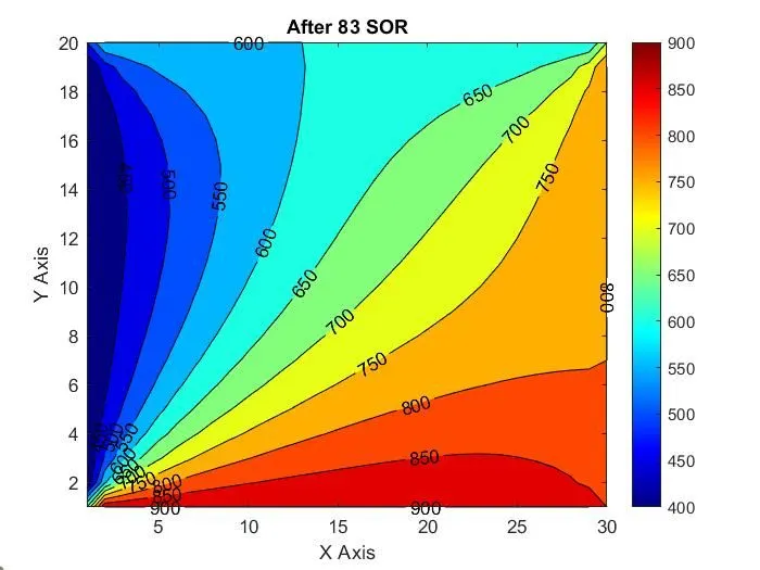
Successive over relaxation iterative solver convergence rate is higher than the jacobi and gauss seidal method for both steady and unsteady state heat conduction equation. The number of iterations required by the successive over relaxation method is less compared to jacobi and gauss seidal method.

Below Table gives the number of iterations required by iterative solvers to converge.

Steady State Heat Conduction Equation
Iterative Solver	No. of iterations
Jacobi	1315
Gauss Seidal	704
Successive over Relaxation	83

Unsteady State Heat Conduction Equation.
Iterative Solver	No. of iterations
Jacobi	3670
Gauss Seidal	2222
Successive over Relaxation	1148

Conclusion:

Implicit method can be used to problems when converged results are needed in less computation time as they are unconditionally stable. With increases in time step size the convergence rate is increased which leads to steady state with less no. of iterations.

Explicit method results time accurate solutions as it is governed by stability criteria when not satisfied it leads to unstable solution and requires more iterations to attain steady state.

But in the code provided above time step size remains constant which is calculated with respect to the stability criteria. Hence for this time step size the explicit scheme leads to faster convergent rate and as the time step size is small the number of iterations increases for implicit scheme which results slower convergence rate.