Week 5.1 - Mid term project - Solving the steady and unsteady 2D heat conduction problem

Aim:

To write a code which solves the 2D heat conduction equation by using the point iterative techniques by the following methods.

1. Jacobi
2. Gauss-seidel
3. Successive over –relaxation

Introduction:

Considering General three dimensional heat conduction equation,

∂T/∂t+ α((∂^2 T)/(∂x^2 )+(∂^2 T)/(∂y^2 )+(∂^2 T)/(∂z^2 ))= 0

The above equation has 2 terms one is time derivative term and another one is spatial derivative and the alpha is thermal diffusivity.

And the two dimensional heat conduction equation,

∂T/∂t+ α((∂^2 T)/(∂x^2 )+(∂^2 T)/(∂y^2 ))= 0

1.Steady State Equation:

• Under this condition the rate of change of temperature remains zero. Therefore the time derivative is equal to zero.
• Steady State 2D Heat Conduction Equation,

(∂^2 T)/(∂x^2 )+(∂^2 T)/(∂y^2 )=0

2.Transient State Equation:

Under this condition both terms are considered therefore the equation will be,

∂T/∂t+ α((∂^2 T)/(∂x^2 )+(∂^2 T)/(∂y^2 ))= 0

Above two equation can be solved in two ways by 3 derivative methods such as Jacobi, Gauss Seidel, SOR.

1. Explicit
2. Implicit

Inputs:

• Assume nx = ny = 10.
• Boundary condition for stady and transient case:
• Top = 600k
• Bottom = 900k
• Left = 400k
• Right = 800k
• Tolerance = 1e-4
• Starting error = 1
• Alpha = 1.2
• Omega = 1.4

Solving the Steady State Equation:

(∂^2 T)/(∂x^2 )+(∂^2 T)/(∂y^2 )=0

Here discretising the equation by applying the central differencing scheme,

T(i.j) = 1/k{((Told(i-1,j)+Told(i+1,j))/(dx^2 ))+((Told(i,j-1)+Told(i,j+1))/(dy^2 )) }
Where,
	k = 2*((dx^2+dy^2)/(dx^2 dy^2 ))

Function code for Jacobi:

function jacobi = jacobi_iter(error,tol,x,y,nx,ny,dx,dy,T,k,Told)
iteration = 1;

while error > tol
    for i = 2:nx-1
        for j = 2:ny-1
            term1 = (Told(i-1,j)+Told(i+1,j))/(dx^2);
            term2 = (Told(i,j-1)+Told(i,j+1))/(dy^2);
            T(i,j) = k*(term1+term2);
        end
    end
    
    jacobi = T(i,j);
    error = max(max(abs(Told - T)));
    Told = T;
    
    iteration = iteration +1;
end
figure(1)
[n,m] = contourf(x,y,T)
clabel(n,m)
colorbar
colormap(jet)
set(gca,'YDIR','reverse')
xlabel('X-Axis')
ylabel('Y-Axis')
title({['Plot for Jacobi Method'],[sprintf('Number of Iteration = %d',iteration)]})
end

Function code for Gauss Seidel:

function gauss_seidel = gs_iter(error,tol,x,y,nx,ny,dx,dy,T,k,Told)
iteration = 1;

while error > tol
    for i = 2:nx-1
        for j = 2:ny-1
            term1 = (T(i-1,j)+Told(i+1,j))/(dx^2);
            term2 = (T(i,j-1)+Told(i,j+1))/(dy^2);
            T(i,j) = k*(term1+term2);
        end
    end
    gauss_seidel = T(i,j);
    error = max(max(abs(Told - T)));
    Told = T;
    
    iteration = iteration +1;
end
figure(1)
[n,m] = contourf(x,y,T)
clabel(n,m)
colorbar
colormap(jet)
set(gca,'YDIR','reverse')
xlabel('X-Axis')
ylabel('Y-Axis')
title({['Plot for Gauss Seidel Method'],[sprintf('Number of Iteration = %d',iteration)]})
end

Function code for SOR:

function sor = sor_iter(error,tol,x,y,nx,ny,dx,dy,T,k,Told,omega)
iteration = 1;
omega = 1.2;
while error > tol
    for i = 2:nx-1
        for j = 2:ny-1
            term1 = (T(i-1,j)+Told(i+1,j))/(dx^2);
            term2 = (T(i,j-1)+Told(i,j+1))/(dy^2);
            T(i,j) = k*(term1+term2);
            T(i,j) = Told(i,j)*(1-omega)+(omega*T(i,j));
        end
    end
    sor = T(i,j);
    error = max(max(abs(Told - T)));
    Told = T;
    
    iteration = iteration +1;
end
figure(1)
[n,m] = contourf(x,y,T)
clabel(n,m)
colorbar
colormap(jet)
set(gca,'YDIR','reverse')
xlabel('X-Axis')
ylabel('Y-Axis')
title({['Plot for SOR Method'],[sprintf('Number of Iteration = %d',iteration)]})
end

Main code:

clear all
close all
clc

%inputs
T_T = 600;
T_B = 900;
T_L = 400;
T_R = 800;

nx = 10;
ny = nx;
x = linspace(0,1,nx);
y = linspace(0,1,ny);
dx = x(2)-x(1);
dy = y(2)-y(1);

T = 300*ones(nx,ny);
T(1,:) = T_T; 
T(ny,:) = T_B;
T(:,1) = T_L;
T(:,nx) = T_R;
T(1,1) = (T_L + T_B)/2;
T(1,ny) = (T_T +T_L)/2;
T(nx,ny) = (T_T + T_R)/2;
T(nx,1) = (T_R +T_B)/2;
Told = T;

k = (dx^2*dy^2)/(2*(dx^2+dy^2));
tol = 1e-4;
error = 1;
itratie_solver = input('enter the desired number with respect to solver');
if itratie_solver==1
    jacobi = jacabi_iter(error,tol,x,y,nx,ny,dx,dy,T,k,Told);
elseif itratie_solver==2
    gauss_seidel = gs_iter(error,tol,x,y,nx,ny,dx,dy,T,k,Told);
elseif itratie_solver==3
    sor = sor_iter(error,tol,x,y,nx,ny,dx,dy,T,k,Told);
end

Results for Solving Steady State Equation:

Plots:

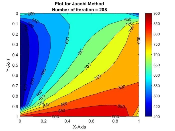
Jacobi Method:

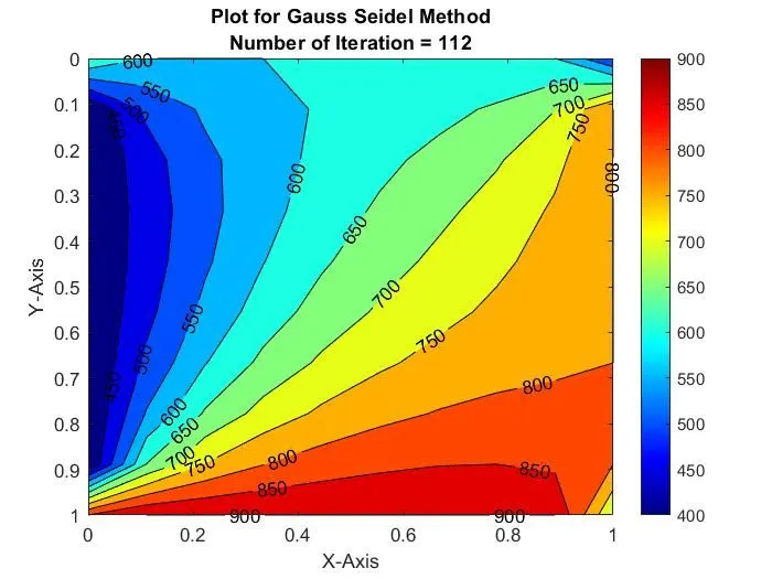
Gauss Seidel Method:

SOR Method:

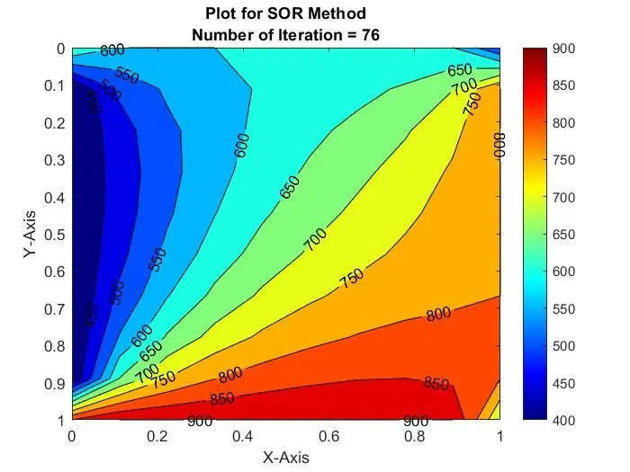
Above plots shows that the SOR method takes less number of iteration to solve the equation when compare to other two methods.

Solving Transient State Equation:

∂T/∂t+ α((∂^2 T)/(∂x^2 )+(∂^2 T)/(∂y^2 ))= 0

This equation can solve by two methods such as implicit method and explicit method.

1.Explicit Method:

• Explicit approach is used in numerical analysis for obtaining numerical approximation to the solution of time dependent ordinary or partial differential as in required in computer simulation of a physical process.
• Here in this equation time derivative terms are calculated using first order differential equation and where as the term 2 has second order derivative terms and elliptical in nature so information needs to be taken from all the points equally, so central differencing scheme is applied for the discretising the term 2.

Term 1 => ∂T/∂t=(T_(i,j)^(n+1)- T_(i,j)^n)/∆t  
Term 2 =>(∂^2 T)/(∂x^2 )+(∂^2 T)/(∂y^2 )=((T_(i∓1,j)^n-2T_(i,j)^n+T_(i-1,j)^n)/(∆x^2 )+(T_(i,j+1)^n-2T_(i,j)^n+T_(i,j-1)^n)/(∆y^2 ))

The discretised equation for 2D heat conduction equation for the explicit form,

T^(n+1) (i,j)= T^n+k1*(T^nold(i+1,j)-2*T^nold(i,j)+T^nold(i-1,j) )+k2*(T^nold(i,j+1)-2*T^nold(i,j)+T^nold(i,j-1) )
Where,
	k1 = α*(dt/(dx^2 ))
	k2 = α*(dt/(dy^2 ))

Main code for Transient heat conduction equation solving by Explicit Method(Jacobi Derivative):

clear all
close all
clc

%inputs
T_T = 600;
T_B = 900;
T_L = 400;
T_R = 800;

nx = 10;
ny = nx;
x = linspace(0,1,nx);
y = linspace(0,1,ny);
dx = x(2)-x(1);
dy = y(2)-y(1);

T = 300*ones(nx,ny);
T(1,:) = T_T; 
T(ny,:) = T_B;
T(:,1) = T_L;
T(:,nx) = T_R;
T(1,1) = (T_L + T_B)/2;
T(1,ny) = (T_T +T_L)/2;
T(nx,ny) = (T_T + T_R)/2;
T(nx,1) = (T_R +T_B)/2;
Told = T;
dt =0.001;
alpha = 1.2;
nt = 500;
k1 = alpha*(dt/(dx^2));
k2 = alpha*(dt/(dy^2));
tol = 1e-4;
error = 1;
iteration = 1;
for k = 1:nt
    while error>tol
    for i = 2:(nx-1)
        for j = 2:(ny-1)
            term1 = Told(i+1,j)-(2*Told(i,j))+Told(i-1,j);
            term2 = Told(i,j+1)-(2*Told(i,j))+Told(i,j-1);
            T(i,j) = Told(i,j)+(k1*term1)+(k2*term2);
        end
    end
     error = max(max(abs(Told-T)));
     Told = T;
     iteration = iteration +1;
    end
end

figure(1)
[n,m] = contourf(x,y,T)
clabel(n,m)
colorbar
colormap(jet)
set(gca,'YDIR','reverse')
xlabel('X-Axis')
ylabel('Y-Axis')
title({['Plot for Explicit Scheme'],[sprintf('Number of Iteration = %d',iteration)]})

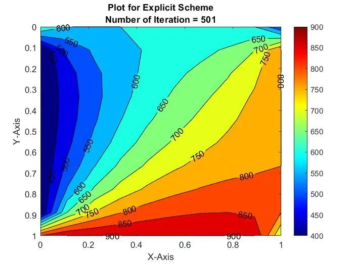
Results for solving Transient State Equation by Explicit Method:

Plot:

2.Implicit Method:

• Implicit approach is used in numerical analysis for obtaining numerical approximations to the solution of time dependent ordinary or partial differential equation as in required in computer simulation or physical process.
• Here in this equation time derivative terms are calculated using first order differential equation and where as the term 2 has second order derivative terms and elliptical in nature , so central differencing method is allied for dicretising the term 2.

Term 1 => ∂T/∂t=(T_(i,j)^(n+1)- T_(i,j)^n)/∆t  
Term 2 =>(∂^2 T)/(∂x^2 )+(∂^2 T)/(∂y^2 )=((T_(i∓1,j)^n-2T_(i,j)^n+T_(i-1,j)^n)/(∆x^2 )+(T_(i,j+1)^n-2T_(i,j)^n+T_(i,j-1)^n)/(∆y^2 ))

The discretised equation for 2D heat conduction equation for the explicit form,

T^(n+1) (i,j)= T^n+[k1*(T^nold(i+1,j)-2*T^nold(i,j)+T^nold(i-1,j))]^(n+1)+[k2*(T^nold(i,j+1)-2*T^nold(i,j)+T^n old(i,j-1))]^(n+1)
Where,
	k1 = α*(dt/(dx^2 ))
	k2 = α*(dt/(dy^2 ))

The above equation is solved by using different iterative methods such as Jacobi, Gauss seidel and SOR method.

In Jacobi method, the unknowns on the RHS are assumed to have an initial value, i.e T at ‘n+1’ at all nodes is assumed. Using the equation, then the LHS is calculated. On the next value of i, j similar method is applied to calculate LHS. Thus in first iteration, value of T for time ‘n+1’ is calculated at all nodes. The difference between T at ‘n+1’ which is obtained and T at ‘n+1’ which was assumed previously is taken. If it is greater than a specified tolerance value, iterations are carried out to calculate T at ‘n+1’. But in the second iteration, T at ‘n+1’ I assumed as the value of T which was obtained in the previous iteration.

Equation for Jacobi method in code:

term1 =1/(1+(2*k1)+(2*k2)); 
term2 = k1*term1;
term3 = k2*term1;
term4 = Told(i-1,j)+Told(i+1,j);
term5 = Told(i,j+1)+Told(i,j+1);
T(i,j)=(term1*T_initial(i,j))+(term2*term4)+(term3*term5);

The Gauss Seidel method is similar to the Jacobi method, but the only difference is for the first iteration when the value of T at a particular node is calculated, this updated valus at that node is used to calculate the value at next node.

Equation for Gauss Seidel method in code:

term1 =1/(1+(2*k1)+(2*k2)); 
term2 = k1*term1;
term3 = k2*term1;
term4 = T(i-1,j)+Told(i+1,j);
term5 = T(i,j+1)+Told(i,j+1);
T(i,j)=(term1*T_initial(i,j))+(term2*term4)+(term3*term5);

SOR method can be applied either by using Jacobi or Gauss Seidel but the only difference is consideration of factor called omega (scaling factor) which in turn makes the process faster which the number of iterations required to solve will b decreased.

Equation for SOR method in code:

term1 =1/(1+(2*k1)+(2*k2)); 
term2 = k1*term1;
term3 = k2*term1;
term4 = T(i-1,j)+Told(i+1,j);
term5 = T(i,j+1)+Told(i,j+1);
T(i,j)=(term1*T_initial(i,j))+(term2*term4)+(term3*term5);
T(i,j) = (T_initial(i,j)*(1-omega))+(omega*T_initial(i,j));

Function code for Jacobi: (Implicit)

function implicit_jacobi = implicit_jacobi_iter(error,tol,x,y,nt,nx,ny,T,k1,k2,T_initial,Told)
iteration = 1;
for k = 1:nt
while error > tol
    for i = 2:nx-1
        for j = 2:ny-1
            term1 =1/(1+(2*k1)+(2*k2)); 
            term2 = k1*term1;
            term3 = k2*term1;
            term4 = Told(i-1,j)+Told(i+1,j);
            term5 = Told(i,j+1)+Told(i,j+1);
            T(i,j) =(term1*T_initial(i,j))+(term2*term4)+(term3*term5);
        end
    end
    
    implicit_jacobi = T(i,j);
    error = max(max(abs(Told - T)));
    Told = T;
    
    iteration = iteration +1;
end
end
figure(1)
[n,m] = contourf(x,y,T)
clabel(n,m)
colorbar
colormap(jet)
set(gca,'YDIR','reverse')
xlabel('X-Axis')
ylabel('Y-Axis')
title({['Plot for Implicit Jacobi Method'],[sprintf('Number of Iteration = %d',iteration)]})
end

Function code for Gauss Seidel: (Implicit)

function implicit_gauss_seidel = implicit_gs_iter(error,tol,x,y,nt,nx,ny,T,k1,k2,T_initial,Told)
iteration = 1;
for k = 1:nt
while error > tol
    for i = 2:nx-1
        for j = 2:ny-1
            term1 =1/(1+(2*k1)+(2*k2)); 
            term2 = k1*term1;
            term3 = k2*term1;
            term4 = T(i-1,j)+Told(i+1,j);
            term5 = T(i,j+1)+Told(i,j+1);
            T(i,j) =(term1*T_initial(i,j))+(term2*term4)+(term3*term5);
        end
    end
    
    implicit_gauss_seidel = T(i,j);
    error = max(max(abs(Told - T)));
    Told = T;
    
    iteration = iteration +1;
end
end
figure(1)
[n,m] = contourf(x,y,T)
clabel(n,m)
colorbar
colormap(jet)
set(gca,'YDIR','reverse')
xlabel('X-Axis')
ylabel('Y-Axis')
title({['Plot for Implicit Gauss Seidel Method'],[sprintf('Number of Iteration = %d',iteration)]})
end

Function code for SOR: (Implicit)

function implicit_sor = implicit_sor_iter(error,tol,x,y,nt,nx,ny,T,omega,k1,k2,T_initial,Told)
iteration = 1;
for k = 1:nt
while error > tol
    for i = 2:nx-1
        for j = 2:ny-1
            term1 =1/(1+(2*k1)+(2*k2)); 
            term2 = k1*term1;
            term3 = k2*term1;
            term4 = T(i-1,j)+Told(i+1,j);
            term5 = T(i,j+1)+Told(i,j+1);
            T(i,j) =(term1*T_initial(i,j))+(term2*term4)+(term3*term5);
            T(i,j) = (T_initial(i,j)*(1-omega))+(omega*T_initial(i,j));
        end
    end
    
    implicit_sor = T(i,j);
    error = max(max(abs(Told - T)));
    Told = T;
    
    iteration = iteration +1;
end
end
figure(1)
[n,m] = contourf(x,y,T)
clabel(n,m)
colorbar
colormap(jet)
set(gca,'YDIR','reverse')
xlabel('X-Axis')
ylabel('Y-Axis')
title({['Plot for Implicit SOR Method'],[sprintf('Number of Iteration = %d',iteration)]})
end

Main code for Transient heat conduction equation solving by Implicit Method:

clear all
close all
clc

%inputs
T_T = 600;
T_B = 900;
T_L = 400;
T_R = 800;

nx = 10;
ny = nx;
x = linspace(0,1,nx);
y = linspace(0,1,ny);
dx = x(2)-x(1);
dy = y(2)-y(1);

T = 300*ones(nx,ny);
T(1,:) = T_T; 
T(ny,:) = T_B;
T(:,1) = T_L;
T(:,nx) = T_R;
T(1,1) = (T_L + T_B)/2;
T(1,ny) = (T_T +T_L)/2;
T(nx,ny) = (T_T + T_R)/2;
T(nx,1) = (T_R +T_B)/2;
Told = T;
T_initial = T;
dt =0.01;
alpha = 1.2;
omega =1.4;
nt = 500;
k1 = alpha*(dt/(dx^2));
k2 = alpha*(dt/(dy^2));
tol = 1e-4;
error = 1;
itratie_solver = input('enter the desired number with respect to solver');
if itratie_solver==1
    implicit_jacobi = implicit_jacobi_iter(error,tol,x,y,nt,nx,ny,T,k1,k2,T_initial,Told)
elseif itratie_solver==2
    implicit_gauss_seidel = implicit_gs_iter(error,tol,x,y,nt,nx,ny,T,k1,k2,T_initial,Told)
elseif itratie_solver==3
    implicit_sor = implicit_sor_iter(error,tol,x,y,nt,nx,ny,T,omega,k1,k2,T_initial,Told)
end

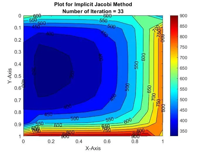
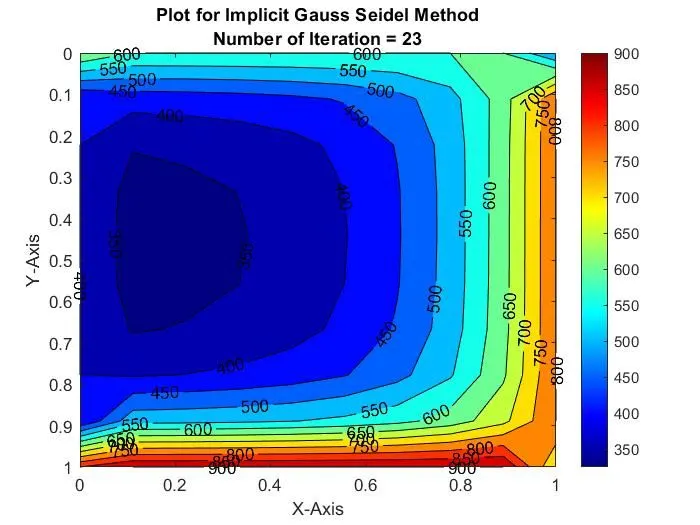
Results for solving Transient State Equation by Implicit Method:

Plot:

Jacobi Method:

Gauss Seidel Method:

SOR Method:

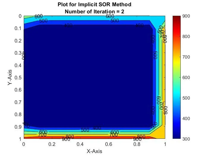
Above plots shows that the SOR method takes less number of iteration to solve the equation when compare to other two methods.

Code Explanation:

• Starting few commands like ‘clear all’, ‘close all’, ‘clc’ are entered to clear any existing data from previous program or command section.
• Enter the input values and boundary condition in the code. Then create a iterative solver to get the required output as our wish.
• Create a sub function code to derive the two dimensional heat conduction equation for each method such as Jacobi, Gauss Seidel and SOR method.
• In that each function code enter the appropriate equation as explained above.
• Then enter the plot command to get required plot in each function code.
• Then call those function code in main code to solve the equation and get the appropriate plot results.
• Save and run the program.
• Repeat the same procedure to the Implicit and Explicit method.