Week 5.1 - Mid term project - Solving the steady and unsteady 2D heat conduction problem
AIM:
To solve the 2D heat conduction equation by using the point iterative technique.
GIVEN:
The boundary conditions
- B(top)=600 K
- B(bottom)=900 K
- B(left)=400 K
- B(right)=800 K
- Absolute error criteria = 1e-4
TO FIND:
- Steady state analysis
- Transient analysis
By the iterative solvers
- Jacobi method
- Gauss- seidal
- SOR
STEADY STATE EQUATIONS:
Steady state is a state where the amount of energy getting inward to an environment is equal to the amount of energy getting outward from the same environment. There is no such system is in steady state initially, and it its not necessary that every unsteady state system should become steady state in a particular period of time.
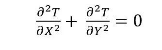
2D heat conduction steady state equation:
Assume,
1. domain length = 1m
2.nx=ny=10,i.e number of nodes.
3.tolerance = 1e-4
4.thermal diffisuvity (alpha)=1.4 m^2/sec
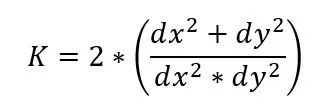
First, discretize the 2D given equation in central differencing scheme,

where ,
Code for three iterative solver method for steady state 2D heat conduction equation:
1.JACOBIAN ITERATIVE SOLVER
Main Program
clear all
close all
clc
%to fix the number of nodes
nx=10;
ny=nx;
x= linspace (0,1,nx);
y=linspace(0,1,nx);
%determine dx and dy
dx=x(2)-x(1);
dy=y(2)-y(1);
k=2*((dx^2+dy^2)/(dx^2*dy^2));
%initaillizing boundary conditions
T=ones(nx,ny);
T(1,:)=900;
T(end,:)=600;
T(:,1)=400;
T(:,end)=800;
Told=T;
%allowing tolerance
tolerance=1e-4;
error=100e-1;
%defning the solvers
iterative_solver = 1;
if iterative_solver==1

    T_jacobi= jacobi_iter_final(error,tolerance,x,y,nx,ny,dx,dy,k,T,Told);
end
Functional Code for jacobian iteration:
function jacobian_iteration = jacobi_iter_final(error,tolerance,x,y,nx,ny,dx,dy,k,T,Told)
jc_iteration=1;
 while(error > tolerance)
     for i= 2:nx-1
         for j= 2:ny-1
            T(i,j)=((Told(i-1,j)+Told(i+1,j))/(k*(dx^2))+(Told(i,j-1)+Told(i,j+1))/(k*(dy^2)));
        end
    end
    error=max(max(abs(Told-T)));
    Told=T;
    jc_iteration=jc_iteration+1;
    jacobian_iteration=figure(1);
    [c,d]=contourf(x,y,T);
    colormap("cool")
    colorbar
    title_text=sprintf('jacobi_iteration=%d',jc_iteration);
    title(title_text)
    xlabel('X AXIS')
    ylabel('Y AXIS')
    clabel(c,d)
    pause(0.03)
 end
end
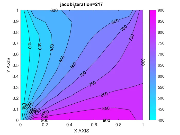
Plot for Jcobian iteration :
GAUSS SEIDAL ITERATIVE SOLVER
2.Main Program for Gauss seidal:
clear all
close all
clc
%to fix the number of nodes
nx=10;
ny=nx;
x= linspace (0,1,nx);
y=linspace(0,1,nx);
%determine dx and dy
dx=x(2)-x(1);
dy=y(2)-y(1);
k=2*((dx^2+dy^2)/(dx^2*dy^2));
%initaillizing boundary conditions
T=ones(nx,ny);
T(1,:)=900;
T(end,:)=600;
T(:,1)=400;
T(:,end)=800;
Told=T;
%allowing tolerance
tolerance=1e-4;
error=100e-1;
%defning the solvers
iterative_solver=2;
if iterative_solver==2
    T_gauss= gauss_iter_final(error,tolerance,x,y,nx,ny,dx,dy,k,T,Told);
end
Function code for gauss seidal :
function gauss_seidal = gauss_iter_final(error,tolerance,x,y,nx,ny,dx,dy,k,T,Told)
gs_iteration=1;
 while(error > tolerance)
     for i= 2:nx-1
         for j= 2:ny-1
            T(i,j)=((T(i-1,j)+Told(i+1,j))/(k*(dx^2))+(T(i,j-1)+Told(i,j+1))/(k*(dy^2)));
        end
    end
    error=max(max(abs(Told-T)));
    Told=T;
    gs_iteration=gs_iteration+1;
    gauss_seidal=figure(2);
    [c,d]=contourf(x,y,T);
    colormap("winter")
    colorbar
    title_text=sprintf('gs iteration=%d',gs_iteration);
    title(title_text)
    xlabel('X AXIS')
    ylabel('Y AXIS')
    clabel(c,d)
    pause(0.03)
end
fprintf('no of iteration i Gs=%d',gs_iteration);
end
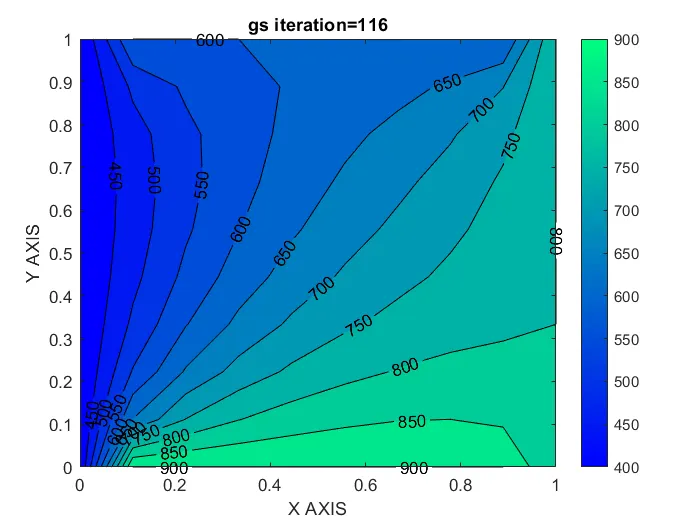
Plot for Gauss seidal iteration:
3.SOR ITERATIVE SOLVER
Main function for SOR iteration:
clear all
close all
clc
%to fix the number of nodes
nx=10;
ny=nx;
x= linspace (0,1,nx);
y=linspace(0,1,nx);
%determine dx and dy
dx=x(2)-x(1);
dy=y(2)-y(1);
k=2*((dx^2+dy^2)/(dx^2*dy^2));
%initaillizing boundary conditions
T=ones(nx,ny);
T(1,:)=900;
T(end,:)=600;
T(:,1)=400;
T(:,end)=800;
Told=T;
%allowing tolerance
tolerance=1e-4;
error=100e-1;
%defning the solvers
iterative_solver = 1;
if iterative_solver==1

    T_SOR= SOR_iter_final(error,tolerance,x,y,nx,ny,dx,dy,k,T,Told);
end
Function code for SOR iteration:
function SOR_iteration = SOR_iter_final(error,tolerance,x,y,nx,ny,dx,dy,k,T,Told)
successive_iteration=1;
omega=1.7;
 while(error > tolerance)
     for i= 2:nx-1
         for j= 2:ny-1
            T(successive_iteration)=(((T(i-1,j)+Told(i+1,j))/(dx^2)+(T(i,j-1)+Told(i,j+1))/(dy^2)))/k;
            T(i,j)=omega*(T(successive_iteration))+(1-omega)*(Told(i,j));
        end
    end
    error=max(max(abs(Told-T)));
    Told=T;
    successive_iteration=successive_iteration+1;
    SOR_iteration=figure(3);
    [c,d]=contourf(x,y,T);
    colormap("cool")
    colorbar
    title_text=sprintf('SOR iteration=%d',successive_iteration);
    title(title_text)
    xlabel('X AXIS')
    ylabel('Y AXIS')
    clabel(c,d)
    pause(0.03)
 end
end
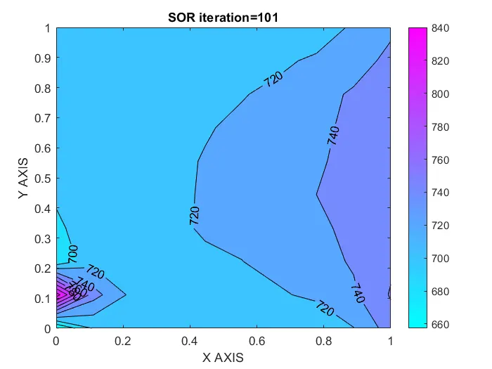
Plot for SOR iteration
UNSTEADY STATE OF 2D HEAT CONDUCTION EQUATION
This Unsteady state is solved by two method
1. Explicit method of approach
2. Implicit method of approach
Explicit method of approach:
General equation for 2D heat conduction equation:
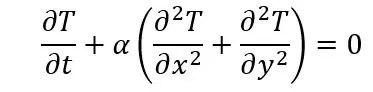
by discretizing it using CDS scheme

where,

This K1 and K2 values are associated with CFL number, CFL is a stability analysis and its value should be less than or equal to 0.5.
In explicit approach the alpha value can be assumed as 1.4 ,so that the heat conduction is faster and can obtain faster results.
EXPLICIT APPROACH OF TRANSIENT STATE
clear all
close all
clc
%to fix the number of nodes
nx=10;
ny=nx;
x= linspace (0,1,nx);
y=linspace(0,1,ny);
%determine dx and dy
dx=x(2)-x(1);
dy=y(2)-y(1);
dt=0.0001;
alpha=1.4;
k1=alpha*(dt/dx^2);
k2=alpha*(dt/dy^2);
CFL=k1+k2;
%initaillizing boundary conditions
T=ones(nx,ny);
T(1,:)=900;
T(end,:)=600;
T(:,1)=400;
T(:,end)=800;
Told=T;
%convergence loop
iteration=1;
for k=1:1400
      for i= 2:nx-1
         for j= 2:ny-1
            T(i,j)=Told(i,j)+ k1*(Told(i-1,j)-2*(Told(i,j))+Told(i+1,j))+k2*(Told(i,j-1)-2*(Told(i,j))+Told(i,j+1));

        end
      end
      Told=T;
      iteration=iteration+1;
       [c,d]=contourf(x,y,T);
    colormap(jet)
    colorbar
    title_text=sprintf('jacobi_iteration=%d',iteration);
    title(title_text)
    xlabel('X AXIS')
    ylabel('Y AXIS')
    clabel(c,d)
    pause(0.003)
end
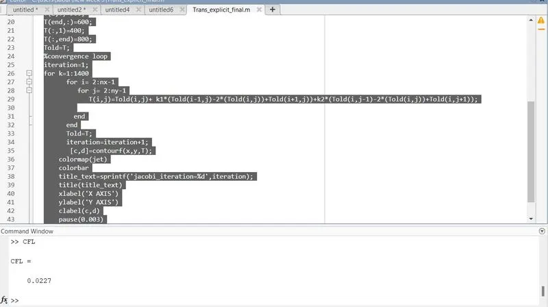
Plot for transient explicit method:
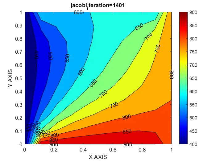
Number of iterations can be varied by changing the values of nx, alpha which directly imact the CFL value , Since the CFL value is 0.02 , which is less than 0.5 the stable solution is obtained.
IMPLICIT APPROACH
As like steady state approach this transient method also can solve by implicit method by using iteration.
2D heat conduction transient state equation:
Discretization is done by

In Implicit method the value of temperature T at n+1 th time step is identified by variying the error and since the variation at n+1 th time step is unknown , we find the value by using iterative solvers.
There are three iterative solver,unlike steady state system
1)jacobi solver
2) gauss seidal solver
3) SOR solver
JACOBIAN ITERATIVE SOLVER
matlab code:
clear all
close all
clc
%to fix the number of nodes
nx=10;
ny=nx;
nt=1200;
x= linspace (0,1,nx);
y=linspace(0,1,nx);
%determine dx and dy
dx=x(2)-x(1);
dy=y(2)-y(1);
dt=0.0001;
alpha=1.4;
k1=alpha*(dt/dx^2);
k2=alpha*(dt/dy^2);
CFL=k1+k2;

%initaillizing boundary conditions
T=ones(nx,ny);
T(1,:)=900;
T(end,:)=600;
T(:,1)=400;
T(:,end)=800;
Told=T;
Tprev=T;
%allowing tolerance
tolerance=1e-4;
%defning the jacobi solvers
iterative_solver = 1;
if iterative_solver==1
    jacobi_iteration=1;
    for c=1:1200
        error=1000;
        while (error>tolerance)
            for i=2:nx-1
                for j=2:ny-1
                    term1= (1+(2*k1)+(2*k2))^(-1);
                    term2= k1*term1;
                    term3= k2*term1;
                    H = (Told(i-1,j)+Told(i+1,j));
                    V = (Told(i,j-1)+Told(i,j+1));
                    T(i,j)= (Tprev(i,j)*term1)+(H*term2)+(V*term3);
                end
            end
            error=max(max(abs(Told-T)));
            Told=T;
            jacobi_iteration=jacobi_iteration+1;
        end
       Tprev=T;
 [c,d]=contourf(x,y,T);
    colormap("jet")
    colorbar
    title_text=sprintf('jacobi_iteration=%d',jacobi_iteration);
   title(title_text)
    xlabel('X AXIS')
    ylabel('Y AXIS')
    clabel(c,d)
    pause(0.03)
    end

end
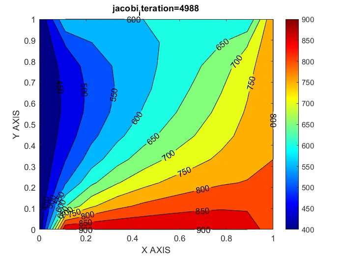
Plot for jacobi:
GAUSS SEIDAL ITERATIVE SOLVER:
MATLAB code for gauss seidal solver:
clear all
close all
clc
%to fix the number of nodes
nx=10;
ny=nx;
nt=1200;
x= linspace (0,1,nx);
y=linspace(0,1,nx);
%determine dx and dy
dx=x(2)-x(1);
dy=y(2)-y(1);
dt=0.0001;
alpha=1.4;
k1=alpha*(dt/dx^2);
k2=alpha*(dt/dy^2);
CFL=k1+k2;

%initaillizing boundary conditions
T=ones(nx,ny);
T(1,:)=900;
T(end,:)=600;
T(:,1)=400;
T(:,end)=800;
Told=T;
Tprev=T;
%allowing tolerance
tolerance=1e-4;
%defning the gauss seidal solvers
iterative_solver = 2;
if iterative_solver==2
    gauss_iteration=2;
    for c=1:1200
        error=1000;
        while (error>tolerance)
            for i=2:nx-1
                for j=2:ny-1
                    term1= (1+(2*k1)+(2*k2))^(-1);
                    term2= k1*term1;
                    term3= k2*term1;
                    H = (T(i-1,j)+Told(i+1,j));
                    V = (T(i,j-1)+Told(i,j+1));
                    T(i,j)= (Tprev(i,j)*term1)+(H*term2)+(V*term3);
                end
            end
            error=max(max(abs(Told-T)));
            Told=T;
            gauss_iteration=gauss_iteration+1;
        end
       Tprev=T;
 [c,d]=contourf(x,y,T);
    colormap("jet")
    colorbar
    title_text=sprintf('gauss_iteration=%d',gauss_iteration);
   title(title_text)
    xlabel('X AXIS')
    ylabel('Y AXIS')
    clabel(c,d)
    pause(0.03)
    end

end
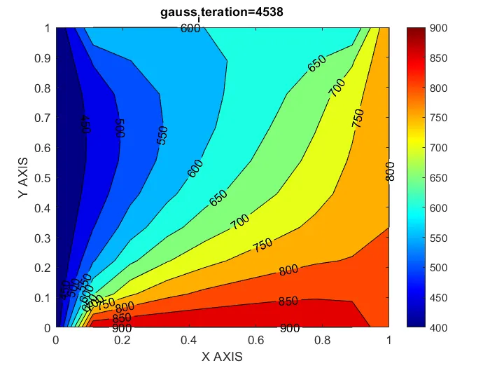
Plot for gauss seidal:
SOR ITERATIVE SOLVER:
MATLAB code for sor iterative solver:
clear all
close all
clc
%to fix the number of nodes
nx=10;
ny=nx;
nt=1200;
x= linspace (0,1,nx);
y=linspace(0,1,nx);
%determine dx and dy
dx=x(2)-x(1);
dy=y(2)-y(1);
dt=0.0001;
alpha=1.4;
k1=alpha*(dt/dx^2);
k2=alpha*(dt/dy^2);
CFL=k1+k2;

%initaillizing boundary conditions
T=ones(nx,ny);
T(1,:)=900;
T(end,:)=600;
T(:,1)=400;
T(:,end)=800;
Told=T;
Tprev=T;
%allowing tolerance
tolerance=1e-4;
omega=1.1;
%defning the SOR solvers
iterative_solver = 3;
if iterative_solver==3
    SOR_iteration=3;
    for c=1:1200
        error=1000;
        while (error>tolerance)
            for i=2:nx-1
                for j=2:ny-1
                    term1= (1+(2*k1)+(2*k2))^(-1);
                    term2= k1*term1;
                    term3= k2*term1;
                    H = (Told(i-1,j)+Told(i+1,j));
                    V = (Told(i,j-1)+Told(i,j+1));
                    T(i,j)= omega*(Tprev(i,j)*term1)+(H*term2)+(V*term3)+(1-omega)*Tprev(i,j);
                end
            end
            error=max(max(abs(Told-T)));
            Told=T;
            SOR_iteration=SOR_iteration+1;
        end
       Tprev=T;
 [c,d]=contourf(x,y,T);
    colormap("jet")
    colorbar
    title_text=sprintf('SOR_iteration=%d',SOR_iteration);
   title(title_text)
    xlabel('X AXIS')
    ylabel('Y AXIS')
    clabel(c,d)
    pause(0.03)
    end

end
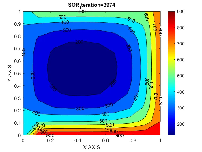
Plot for sor iteration:
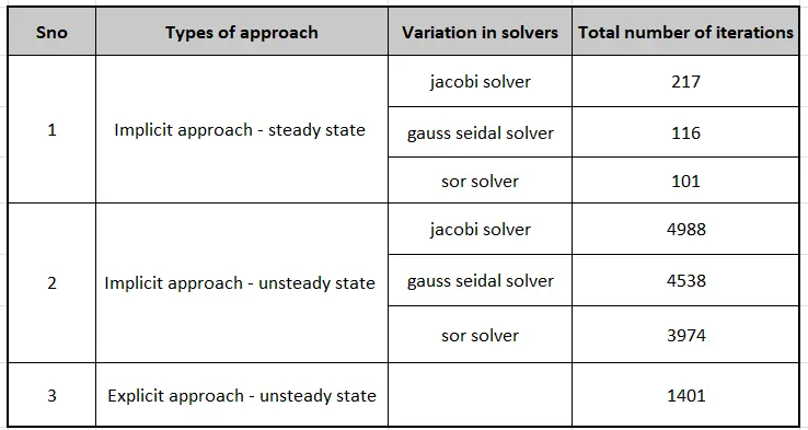
CONCLUSION:
Hints or Notes :
This shows Jacobian iterative solvers take large no of iterations to solve since the value of T is no updated.
Explicit approach in the steady state heat conduction equation is more complex.
Explicit approach mainly accompained by CFL value.
Error value should be within the time loop for implicit approach.
Incase of larger error value makes the simulation time faster.