Week 5.1 - Mid term project - Solving the steady and unsteady 2D heat conduction problem
AIM:- To solve Steady and un-steady 2D Heat conduction Equation by using various Iterative techniques such as Jacobi method, Gauss Sidel method, Successive over relaxation for Implicit and Explicit Schemes by using MATLAB.
GIVEN DATA:-
- Boundary Conditions:
Top Boundary = 600 K
Bottom Boundary = 900 K
Left Boundary = 400 K
Right Boundary = 800 K
- Domain of 1unit square area.
- Assume nx=ny=10; No.of Points along X axis and Y Axis Respectively.
- Initial temperature for all nodes=300 K
THEORY:-
- What is the heat equation?
- Transfer of Heat Energy.
- Steady State: Temperature With respect to time is Constant in Steady State condition.
- Un-steady/Transient state : Temperature With respect to time is changes still reach steady state condition.
2D Heat conduction Equation given as,
`(delT)/(delt)-alpha((delT)/(delx^2)+(delT)/(dely^2))`
The Equation can be written as,
`(delT)/(delt)=alpha((delT)/(delx^2)+(delT)/(dely^2))`
Where,
`alpha=`Thermal Diffussivity in `m^2/s`
Steady State condition(implicit Schemes):
In steady state condition Temperature with respect to time is constant so equation as follows,
`((delT)/(delx^2)+(delT)/(dely^2))=0`
by discretizing equation by central diffrence shemes we get,
`Tp=(1/k)*[(Tl+Tr)/(Deltax^2)+(Tt+Tb)/(Deltay^2)]`
here,
`k=2((Deltax^2+Deltay^2)/(Deltax^2*Deltay^2))`
but we assume `Deltax=Deltay`
so above equation written as,
`Tp=0.25(Tl+Tr+Tt+Tb)`
above equation can be written as,
`Ti,j=0.25(Ti-1,j+Ti+1,j+Ti,j+1+Ti,j-1)`
MATLAB CODE for steady state equation (Jacobi Iteration):
clear all
close all
clc

% To solve stedy state 2D Heat conduction equation  by using Jacobi method
% Inputs
% No. of grid points

nx=10;
ny=nx;

x=linspace(0,1,nx);
dx=x(2)-x(1);
y=linspace(0,1,ny);
dy=dx;

% absolute error criteria>tolerance

error=8e9;
tolerance=1e-4;

% Defining boundary conditions

T_L=400;
T_T=600;
T_R=800;
T_B=900;

T=ones([nx,ny])*300;

% Applying given boundary conditions

T(1,1:nx)=T_T;
T(ny,1:nx)=T_B;
T(2:ny-1,1)=T_L;
T(2:ny-1,nx)=T_R;

% calculate Average Temperatures at Corners

T(1,1)=(T_T+T_L)/2;
T(nx,ny)=(T_R+T_B)/2;
T(1,ny)=(T_T+T_R)/2;
T(nx,1)=(T_L+T_B)/2;

% Assgning new value to T
T_initial=T;
T_old=T;

% calculating 2D state Heat conduction Equation by jacobi method
iterative_solver=1;
if iterative_solver==1
    jacobi_iteration=1;
    while(error>tolerance)

        for i= 2:nx-1
            for j=2:ny-1
                T(i,j)=0.25*((T_old(i,j-1)+T_old(i,j+1)+T_old(i-1,j)+T_old(i+1,j)));
            end
        end
        error=max(max(abs(T_old-T)));
        T_old=T;
        jacobi_iteration=jacobi_iteration+1;
    end
end

% plotting
figure(1)
contourf(x,y,T)
clabel(contourf(x,y,T))
colorbar
colormap("jet")
set(gca,'ydir','reverse')


xlabel('X-axis')
ylabel('Y-axis')
title(sprintf('No of jacobi iterations=%d',jacobi_iteration));
pause(0.03);
EXPLAINATION OF Above code:-
Step-1:- We are getting grid points in x Axis and Y Axis by assuming number of grid points nx and ny for thin 2D plate of area of unit square as 10.
Step-2:- We are getting linear spaced element for X and Y Direction by using linspace Command.
Step-3:- Defined Absolute error criteria as 'error>Tolerance'. also assume error value as '8e9'. and Given tolerance value is '1e-4'. also define the boundary condition as Temperature is 300k.
Step-4:- we are using for loop and While loop for calculating Temperature values for each Iterations before the loop Completion we can also calculate the absolute errors and then update the T_old=T;
Step-5:- by using 'contourf' command we can plot Temperature values for each iteration with respect to X and Y Direction. 'clabel' command used for label the temperature values , colorbar command used for showing Temperature region colorwise and colormap command used for showing color templets in Plot.
OUTPUT for steady state equation (Jacobi Iteration):
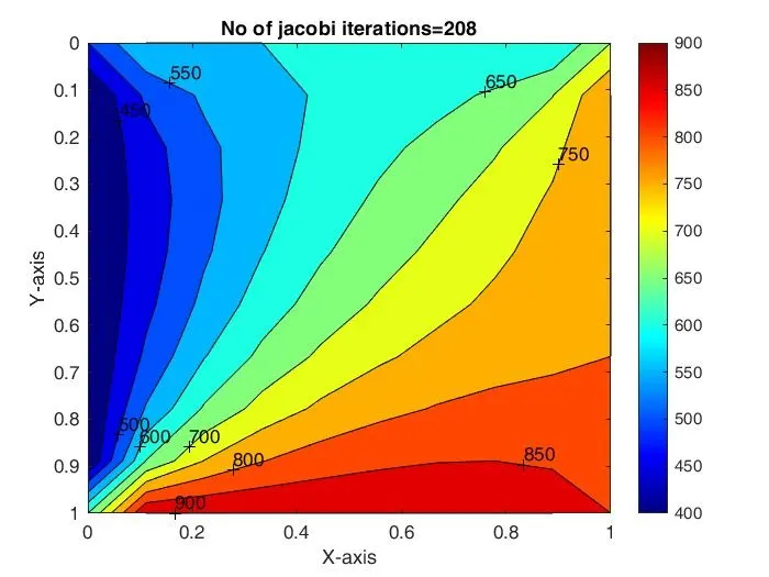
Fig.1 OUTPUT for steady state equation (Jacobi Iteration)
MATLAB CODE for steady state equation (Gauss Sidel Iteration):-
clear all
close all
clc

% solving 2D Heat convection Equation by using Gauss Siedal Method
% Inputs
% No of grid points

nx=10;
ny=nx;

x=linspace(0,1,nx);
dx=x(2)-x(1);
y=linspace(0,1,ny);
dy=dx;

% absolute error criteria>tolerance

error=8e9;
tolerance=1e-4;

% Defining boundary conditions

T_L=400;
T_T=600;
T_R=800;
T_B=900;

T=ones([nx,ny])*300;

% Applying given boundary conditions
T(1,1:nx)=T_T;
T(ny,1:nx)=T_B;
T(2:ny-1,1)=T_L;
T(2:ny-1,nx)=T_R;

% calculate Average Temperatures at Corners

T(1,1)=(T_T+T_L)/2;
T(nx,ny)=(T_R+T_B)/2;
T(1,ny)=(T_T+T_R)/2;
T(nx,1)=(T_L+T_B)/2;

% Assgning new value to T
T_initial =T;
T_old=T;

% calculating 2D state Heat conduction Equation by Gauss Siedal method
iterative_solver=2;
if iterative_solver==2
    GS_iteration=1;
    while(error>tolerance)

        for i= 2:nx-1
            for j=2:ny-1
                T(i,j)=0.25*((T(i,j-1)+T_old(i,j+1)+T(i-1,j)+T_old(i+1,j)));
            end
        end
        error=max(max(abs(T_old-T)));
        T_old=T;
        GS_iteration= GS_iteration+1;
    end
end

% plotting
figure(1)
contourf(x,y,T)
clabel(contourf(x,y,T))
colorbar
colormap(jet)
set(gca,'ydir','reverse')


xlabel('X-axis')
ylabel('Y-axis')
title(sprintf('No of GS iterations=%d',GS_iteration));
pause(0.03);
- OUTPUT for steady state equation (Gauss sidel iteration method ):
No of iteration by using Gauss sidel iteration method is 112.
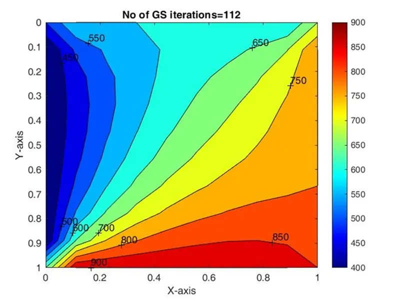
Fig.2 OUTPUT for steady state equation (Gauss sidel iteration method )
- MATLAB CODE for 2D Heat convection Equation by using Successive over relaxation Method:-
clear all

close all

clc


% solving 2D Heat convection Equation by using Successive over relaxation Method

% Inputs

% No of grid points


nx=10;

ny=nx;


x=linspace(0,1,nx);

dx=x(2)-x(1);

y=linspace(0,1,ny);

dy=dx;


% absolute error criteria>tolerance


error=8e9;

tolerance=1e-4;

omega=1.2;


% Defining boundary conditions


T_L=400;

T_T=600;

T_R=800;

T_B=900;


T=ones([nx,ny])*300;


% Applying given boundary conditions

T(1,1:nx)=T_T;

T(ny,1:nx)=T_B;

T(2:ny-1,1)=T_L;

T(2:ny-1,nx)=T_R;


% calculate Average Temperatures at Corners


T(1,1)=(T_T+T_L)/2;

T(nx,ny)=(T_R+T_B)/2;

T(1,ny)=(T_T+T_R)/2;

T(nx,1)=(T_L+T_B)/2;


% Assgning new value to T

T_initial =T;

T_old=T;


% calculating 2D state Heat conduction Equation by Successive over relaxation method

iterative_solver=3;

if iterative_solver==3

    SOR_iteration=1;

    while(error>tolerance)

         for i= 2:nx-1

            for j=2:ny-1

                T(i,j)=(1-omega)*(T_old(i,j))+(omega)*0.25*((T(i,j-1)+T_old(i,j+1)+T(i-1,j)+T_old(i+1,j)));

            end

        end

        error=max(max(abs(T_old-T)));

        T_old=T;

        SOR_iteration= SOR_iteration+1;

    end

end


% plotting

figure(1)

contourf(x,y,T)

clabel(contourf(x,y,T))

colorbar

colormap(jet)

set(gca,'ydir','reverse')


xlabel('X-axis')

ylabel('Y-axis')

title(sprintf('No of SOR iterations=%d',SOR_iteration));

pause(0.03);
- OUTPUT for 2D Heat convection Equation by using Successive over relaxation Method:-
No.of iterations for Successive over relaxation Method is 76.
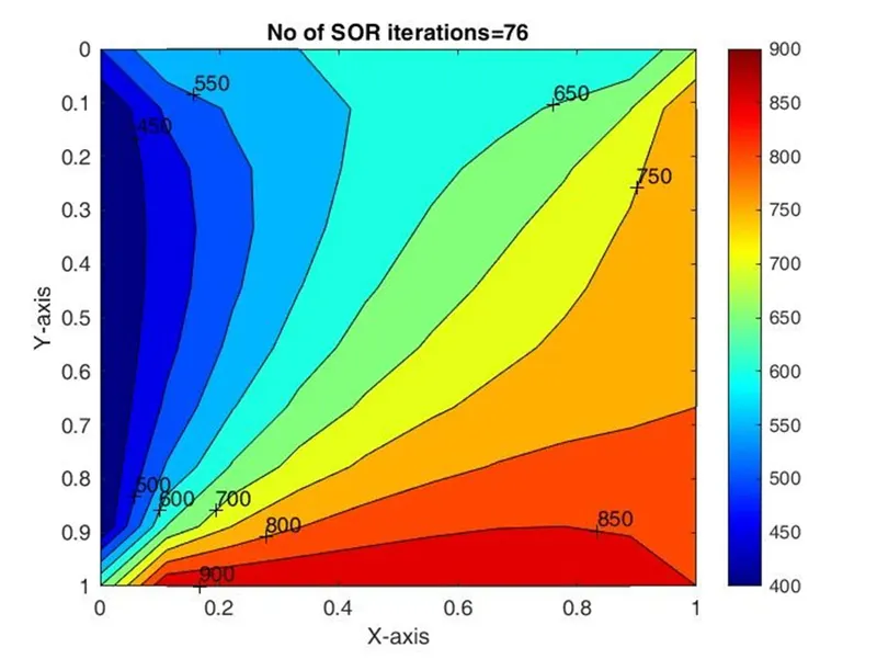
Fig. 3. 2D Heat convection Equation by using Successive over relaxation Method
- MATLAB CODE for 2D Heat convection Equation implicit scheme by using Jacobi Method:-
clear all
close all
clc

% solving Unsteady 2D Heat convection Equation impicit scheme by using Jacobi Method
% Inputs
% No of grid points

nx=10;
ny=nx;
nt=1400;
alpha=1.1;

x=linspace(0,1,nx);
dx=x(2)-x(1);
y=linspace(0,1,ny);
dy=dx;

% absolute error criteria>tolerance

error=8e9;
tolerance=1e-4;
dt=1e-3;

% Defining boundary conditions

T_L=400;
T_T=600;
T_R=800;
T_B=900;

T=ones([nx,ny])*300;

% Applying given boundary conditions
T(1,1:nx)=T_T;
T(ny,1:nx)=T_B;
T(2:ny-1,1)=T_L;
T(2:ny-1,nx)=T_R;

% calculate Average Temperatures at Corners

T(1,1)=(T_T+T_L)/2;
T(nx,ny)=(T_R+T_B)/2;
T(1,ny)=(T_T+T_R)/2;
T(nx,1)=(T_L+T_B)/2;

% Assgning new value to T
T_initial =T;
T_old=T;

% calculating 2D Unsteady state Heat conduction Equation by Jacobi method
k1=alpha*(dt/(dx^2));
k2=alpha*(dt/(dy^2));

Jacobi_iteration=1;
for k=1:nt
    error=8e9;
    while(error>tolerance)
         for i=2:nx-1
            for j=2:ny-1
                Term_1=1/(1+(2*k1)+(2*k2));
                Term_2=k1*Term_1;
                Term_3=k2*Term_1;
                H=(T_old(i-1,j))+(T_old(i+1,j));
                V=(T_old(i,j+1))+(T_old(i,j-1));

                T(i,j)=(T_initial(i,j)*Term_1)+(H*Term_2)+(V*Term_3);

            end
         end

        error=max(max(abs(T_old-T)));
        T_old=T;
        Jacobi_iteration= Jacobi_iteration+1;
    end
    T_initial=T;


% plotting
figure(1)
contourf(x,y,T)
clabel(contourf(x,y,T))
colorbar
colormap(jet)
set(gca,'ydir','reverse')


xlabel('X-axis')
ylabel('Y-axis')
title(sprintf('No of Unsteady Jacobi (implicit) iterations=%d',Jacobi_iteration));
pause(0.03);
end
- OUTPUT for 2D Heat convection Equation implicit scheme by using Jacobi Method:
No.of iterations for implicit scheme by using Jacobi Method is 3880.
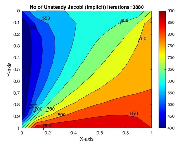
Fig. 4. 2D Heat convection Equation implicit scheme by using Jacobi Method.
- MATLAB CODE for 2D Heat convection Equation implicit scheme by using Gauss Siedel Method
clear all
close all
clc

% solving Unsteady 2D Heat convection Equation impicit scheme by using Gauss Siedal Method
% Inputs
% No of grid points

nx=10;
ny=nx;
nt=1400;
alpha=1.1;

x=linspace(0,1,nx);
dx=x(2)-x(1);
y=linspace(0,1,ny);
dy=dx;

% absolute error criteria>tolerance

error=8e9;
tolerance=1e-4;
dt=1e-3;

% Defining boundary conditions

T_L=400;
T_T=600;
T_R=800;
T_B=900;

T=ones([nx,ny])*300;

% Applying given boundary conditions
T(1,1:nx)=T_T;
T(ny,1:nx)=T_B;
T(2:ny-1,1)=T_L;
T(2:ny-1,nx)=T_R;

% calculate Average Temperatures at Corners

T(1,1)=(T_T+T_L)/2;
T(nx,ny)=(T_R+T_B)/2;
T(1,ny)=(T_T+T_R)/2;
T(nx,1)=(T_L+T_B)/2;

% Assgning new value to T
T_initial =T;
T_old=T;

% calculating 2D Unsteady state Heat conduction Equation by Gauss Sidel method
k1=alpha*(dt/(dx^2));
k2=alpha*(dt/(dy^2));

GS_iteration=1;
for k=1:nt
    error=8e9;
    while(error>tolerance)
         for i=2:nx-1
            for j=2:ny-1
                Term_1=1/(1+(2*k1)+(2*k2));
                Term_2=k1*Term_1;
                Term_3=k2*Term_1;
                H=(T(i-1,j))+(T_old(i+1,j));
                V=(T(i,j+1))+(T_old(i,j-1));

                T(i,j)=(T_initial(i,j)*Term_1)+(H*Term_2)+(V*Term_3);

            end
         end

        error=max(max(abs(T_old-T)));
        T_old=T;
        GS_iteration= GS_iteration+1;
    end
    T_initial=T;


% plotting
figure(1)
contourf(x,y,T)
clabel(contourf(x,y,T))
colorbar
colormap(jet)
set(gca,'ydir','reverse')


xlabel('X-axis')
ylabel('Y-axis')
title(sprintf('No of Unsteady Gauss sidel (implicit) iterations=%d',GS_iteration));
pause(0.03);
end
- OUTPUT for 2D Heat convection Equation implicit scheme by using Gauss Siedel Method:
No.of iterations for implicit scheme by using Gauss Siedel Method is 3612.
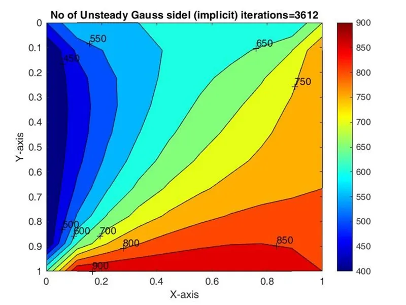
Fig.5. 2D Heat convection Equation implicit scheme by using Gauss Siedel Method
- MATLAB CODE for Unsteady 2D Heat convection Equation impicit scheme by using Successive over relaxation Method:-
clear all
close all
clc

% solving Unsteady 2D Heat convection Equation impicit scheme by using Successive over relaxation Method
% Inputs
% No of grid points

nx=10;
ny=nx;
nt=1400;
alpha=1.1;

x=linspace(0,1,nx);
dx=x(2)-x(1);
y=linspace(0,1,ny);
dy=dx;

% absolute error criteria>tolerance

error=8e9;
tolerance=1e-4;
dt=1e-3;
omega=1.1;


% Defining boundary conditions

T_L=400;
T_T=600;
T_R=800;
T_B=900;

T=ones([nx,ny])*300;

% Applying given boundary conditions
T(1,1:nx)=T_T;
T(ny,1:nx)=T_B;
T(2:ny-1,1)=T_L;
T(2:ny-1,nx)=T_R;

% calculate Average Temperatures at Corners

T(1,1)=(T_T+T_L)/2;
T(nx,ny)=(T_R+T_B)/2;
T(1,ny)=(T_T+T_R)/2;
T(nx,1)=(T_L+T_B)/2;

% Assgning new value to T
T_initial =T;
T_old=T;
T_end=T;

% calculating 2D Unsteady state Heat conduction Equation by Successive over relaxation method
k1=alpha*(dt/(dx^2));
k2=alpha*(dt/(dy^2));

SOR_iteration=1;
for k=1:nt
    error= 8e9;
    while(error>tolerance)

         for i=2:nx-1
            for j=2:ny-1
                Term_1=1/(1+(2*k1)+(2*k2));
                Term_2=k1*Term_1;
                Term_3=k2*Term_1;
                H=(T(i-1,j))+(T_old(i+1,j));
                V=(T(i,j+1))+(T_old(i,j-1));

                T(i,j)=(T_initial(i,j)*Term_1)+(H*Term_2)+(V*Term_3);
                T_end(i,j)=(1-omega)*(T_old(i,j))+(T(i,j)*omega);

            end
         end
         error=max(max(abs(T_old-T)));
         T_old=T_end;
         SOR_iteration= SOR_iteration+1;
    end
    T_initial=T_end;

% plotting
figure(1)
contourf(x,y,T)
clabel(contourf(x,y,T))
colorbar
colormap(jet)
set(gca,'ydir','reverse')


xlabel('X-axis')
ylabel('Y-axis')
title(sprintf('No of Unsteady Successive over relaxtaion (implicit) iterations=%d',SOR_iteration));
pause(0.03);
end
- OUTPUT for Unsteady 2D Heat convection Equation impicit scheme by using Successive over relaxation Method
No.of iterations for Unsteady 2D Heat convection Equation impicit scheme by using Successive over relaxation Method is 3290.
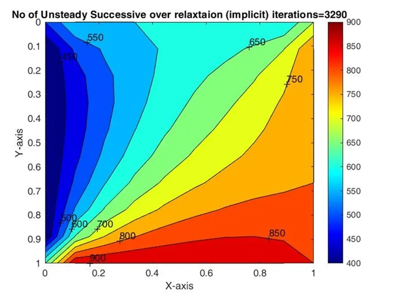
Fig.6. Unsteady 2D Heat convection Equation impicit scheme by using Successive over relaxation Method
- Explicit Scheme Unstedy state Condition:-
Unstedy State equation:
equation for unsteady state is given as,
`(delT)/(delt)=alpha((del^2T)/(delx^2)+(del^2T)/(dely^2))`
After descretizing the above equation we get,
`(T_p^(n+1)-T_p^n)/(Deltat)=alpha((T_L-2T_p+T_R)/(Deltax^2)+(T_T-2T_P+T_B)/(Deltay^2))`
by simplifying above equation,
`(T_p^(n+1))=T_p^n+K_1(T_L-2T_P+T_R)^n+K_2(T_T-2T_P+T_B)^n`
Where,
`K_1=alpha*((Deltat)/(Deltax^2))`
`K_2=alpha*((Deltat)/(Deltay^2))`
For betterment of code we can write equation as,
`(T_(i,j))=T_(i,j)+K_1(T_(i-1,j)-2T_(i,j)+T_(i+1,j))+K_2(T_(i,j+1)-2T_(i,j)+T_(i,j-1))`
- MATLAB CODE for Unsteady 2D Heat convection Equation Explicit Scheme.
clear all
close all
clc

% solving Unsteady 2D Heat convection Equation explicit scheme
% Inputs
% No of grid points

nx=10;
ny=nx;
nt=1400;
alpha=1.1;

x=linspace(0,1,nx);
dx=x(2)-x(1);
y=linspace(0,1,ny);
dy=dx;

% absolute error criteria>tolerance

error=8e9;
tolerance=1e-4;
dt=1e-3;


% Defining boundary conditions

T_L=400;
T_T=600;
T_R=800;
T_B=900;

T=ones([nx,ny])*300;

% Applying given boundary conditions
T(1,1:nx)=T_T;
T(ny,1:nx)=T_B;
T(2:ny-1,1)=T_L;
T(2:ny-1,nx)=T_R;

% calculate Average Temperatures at Corners

T(1,1)=(T_T+T_L)/2;
T(nx,ny)=(T_R+T_B)/2;
T(1,ny)=(T_T+T_R)/2;
T(nx,1)=(T_L+T_B)/2;

% Assgning new value to T
T_initial =T;
T_old=T;

% calculating 2D Unsteady state Heat conduction Equation by Explicit method
k1=alpha*(dt/(dx^2));
k2=alpha*(dt/(dy^2));
iterative_solver=1;
if iterative_solver==1
    unsteady_explicit=1;
    for k=1:nt
    error= 8e9;
    while(error>tolerance)
        for i=2:nx-1
            for j=2:ny-1
                Term_1=T_old(i,j);
                Term_2=k1*(T_old(i+1,j)-2*T_old(i,j)+T_old(i-1,j));
                Term_3=k2*(T_old(i,j+1)-2*T_old(i,j)+T_old(i,j-1));


                T(i,j)=Term_1+Term_2+Term_3;

            end
         end
         error=max(max(abs(T_old-T)));
         T_old=T;
         unsteady_explicit= unsteady_explicit+1;
    end
   end
end

% plotting
figure(1)
contourf(x,y,T)
clabel(contourf(x,y,T))
colorbar
colormap(jet)
set(gca,'ydir','reverse')


xlabel('X-axis')
ylabel('Y-axis')
title(sprintf('No of Unsteady Explicit iterations=%d',unsteady_explicit));
pause(0.03);
- OUTPUT for Unsteady 2D Heat convection Equation Explicit scheme
No.of iterations for Unsteady 2D Heat convection Equation Explicit scheme Method is 1941.
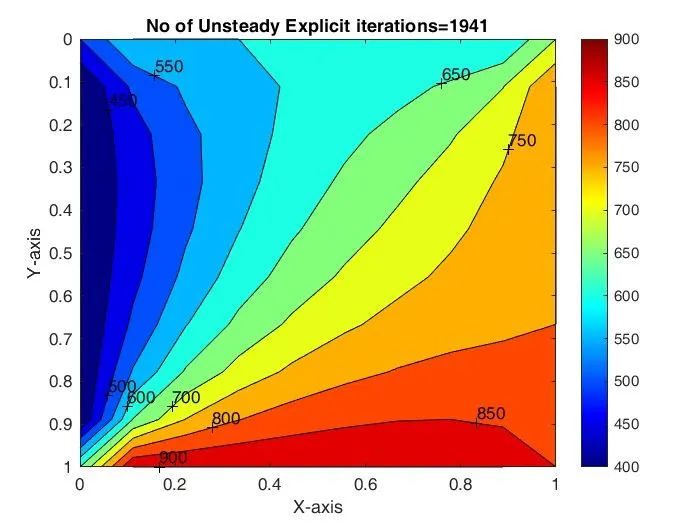
Fig.7. OUTPUT for Unsteady 2D Heat convection Equation Explicit scheme
CONCLUSION:-
No. of iteration for type of Scheme used.
- Implicit Steady state Analysis
- Jacobi=208
- Gauss Sidel=112
- Successive Over-relaxtaion=76
- Implicit Un-Steady state Analysis
- Jacobi=3880
- Gauss Sidel=3612
- Successive Over-relaxtaion=3290
- Explicit Un-Steady state Analysis
- Un-Steady state=1941
We can conclude that,
- While comparing Steady state and Unstedy State, Steady state takes less time and it require less No. of iterations.
- Successive Over-relaxtaion Method is more convinient because it requires less No of iteration for getting Result in both Implicit and Explicit Schemes, compared to Jacobi and Gauss Sidel method.