Challenge

Week 5.1 - Mid term project - Solving the steady and unsteady 2D heat conduction problem

RRagam Vinay Kumar4 Jun 2022

1. Steady state analysis & Transient State Analysis

Solve the 2D heat conduction equation by using the point iterative techniques that were taught in the class. The Boundary conditions for the problem are as follows;

Top Boundary = 600 K

Bottom Boundary = 900 K

Left Boundary = 400 K

Right Boundary = 800 K

You will implement the following methods for solving implicit equations.

1. Jacobi

2. Gauss-seidel

3. Successive over-relaxation

Your absolute error criteria is 1e-4

EXPLANATION :

The heat equation is a partial differential equation that describes how the distribution of some quantity evolves over time in a solid medium , as it spontaneously flows from places where it is higher towards places where it is lower.

For a function u(x,y,z,t) of three spatial variables (x,y,z) and the time variable t, the heat equation is

`partialu/partialt = alpha(partial^2u/partialx^2+partial^2u/partialy^2 +partial^2u/partialz^2)`

TYPES OF HEAT CONDUCTION SCHEMES :

This transfer of heat energy may occur under two conditiions

1. Steady state condition.

2.Unsteady state condition.

Unsteady state conditions are a precursor to stead sate conditions . No system exists initiallly under steady state conditions. Some time must pass , after transfer is initiated,before the system reaches steady state. During that perriod of transition the system is under unsteady state conditions..

T_L = Left boundary

T_T = Top boundary

T_P = Poinnt boundary

T_B = Bottom boundary

T_R = Right boundary

GOVERNING EQUATIONS :

In order to solve the 2D heat conduction problem, the governing equations for respective conditions with respect to cartesian coordinates should be discretized to enter that in a code which is given under MAIN PROGGRAM below.

MAIN PROGRAM :

Below there is a sequence of seven individual proograms ,starting with implicit scheme of steady and unsteady state conditions for three iterative methods

Jacobi,Gauss-siedel and SOR followed by explicit scheme for unsteady conditions.

IMPLICIT SCHEME STEADY STATE CONDITION PROGRAM :

Steady state equation discretization :

In steady state conditions, the amount of heat entering any regiion of an object is equal to the amount of heat coming out,

`partial^2T/partialx^2 + partial^2T/partialy^2 = 0`

by discretizind the equation above it becomes,

`T_p = 1/k[T_L +T_R/trianglex^2+T_T+T_B/triangley^2]`

here ,the value of k is,

`K = 2(trianglex^2 + triangley^2/trianglex^2 triangle y^2)`

which can also be written as,

`0.25*(T_L+T_R+T_T+T_B)`

JACOBI ITERATION :

% solving steady and unsteady 2D heat conduction problem
% steady state condition
% iterative solver-jacobi,Gauss-seidel,Relaxation methods

clear all
close all
clc

% initial conditions
%L = 1;
nx = 10;
ny = nx;
x = linspace(0,1,nx);
y = linspace(0,1,ny);
dx = x(2)-x(1);
dy = dx;

% Abosolute error criteria > tolerance
error = 9e9;
tolerance = 1e-4;

% defining boundary conditions
T_L = 400;
T_T = 600;
T_R = 800;
T_B = 900;

T = 300*ones(nx,ny);

T(2:ny-1,1) = T_L;
T(2:ny-1,nx) = T_R;
T(1,2:nx-1) = T_T;
T(ny,2:nx-1) = T_B;

% calculating average temperatures at corners

T(1,1) = (T_T+T_L)/2;
T(nx,ny) = (T_R+T_B)/2;
T(1,ny) = (T_T+T_R)/2;
T(nx,1) = (T_L+T_B)/2;

% assigning  original values for T
T_intial = T;
T_old = T;


% JACOBI ITERATIVE METHOD
iterative_solver = 1;

if iterative_solver == 1
    jacobi_iteration = 1;

    while(error > tolerance)
    

    for i = 2:nx-1

        for j = 2:ny-1
            T(i,j) = 0.25*(T_old(i-1,j)+T_old(i+1,j)+T_old(i,j-1)+T_old(i,j+1));
        end
    end
        error =  max(max(abs(T_old-T)));
        T_old = T;
        jacobi_iteration = jacobi_iteration+1;
    end
end



% plotting
figure(1);
contourf(x,y,T,'ShowText','on');
clabel(contourf(x,y,T))
colorbar;
colormap(jet);
set(gca,'ydir','reverse')
xlabel('x-axis')
ylabel('y-axis')
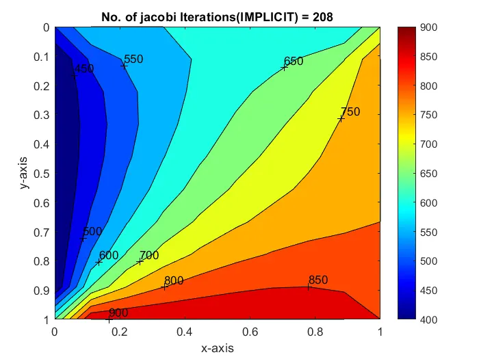
title(sprintf('No. of jacobi Iterations(IMPLICIT) = %d',jacobi_iteration));
pause(0.1);

PLOT :

GAUSS-SIEDEL ITERATION :

% solving steady and unsteady 2D heat conduction problem
% steady state condition
% iterative solver-jacobi,Gauss-seidel,Relaxation methods

clear all
close all
clc

% initial conditions
%L = 1;
nx = 10;
ny = nx;
x = linspace(0,1,nx);
y = linspace(0,1,ny);
dx = x(2)-x(1);
dy = dx;

% Abosolute error criteria > tolerance
error = 9e9;
tolerance = 1e-4;

% defining boundary conditions
T_L = 400;
T_T = 600;
T_R = 800;
T_B = 900;

T = 300*ones(nx,ny);

T(2:ny-1,1) = T_L;
T(2:ny-1,nx) = T_R;
T(1,2:nx-1) = T_T;
T(ny,2:nx-1) = T_B;

% calculating average temperatures at corners

T(1,1) = (T_T+T_L)/2;
T(nx,ny) = (T_R+T_B)/2;
T(1,ny) = (T_T+T_R)/2;
T(nx,1) = (T_L+T_B)/2;

% assigning  original values for T
T_intial = T;
T_old = T;


% GAUSS-SEIDEL ITERATIVE METHOD
iterative_solver = 2;

if iterative_solver == 2
    gauss_iteration = 1;

    while(error > tolerance)
    

    for i = 2:nx-1

        for j = 2:ny-1
            T(i,j) = 0.25*(T(i-1,j)+T_old(i+1,j)+T_old(i,j-1)+T_old(i,j+1));
        end
    end
        error =  max(max(abs(T_old-T)));
        T_old = T;
        gauss_iteration = gauss_iteration+1;
    end
end



% plotting
figure(1);
contourf(x,y,T,'ShowText','on');
clabel(contourf(x,y,T))
colorbar;
colormap(jet);
set(gca,'ydir','reverse')
xlabel('x-axis')
ylabel('y-axis')
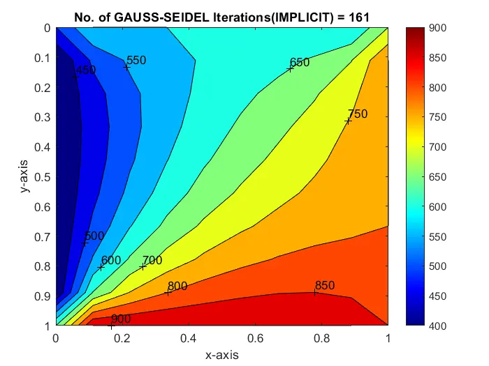
title(sprintf('No. of GAUSS-SEIDEL Iterations(IMPLICIT) = %d',gauss_iteration));
pause(0.03);

PLOT :

SUCCESSIVE OVER-RELAXATION :

% solving steady and unsteady 2D heat conduction problem
% steady state condition
% iterative solver-jacobi,Gauss-seidel,Relaxation methods

clear all
close all
clc

% initial conditions
%L = 1;
nx = 10;
ny = nx;
x = linspace(0,1,nx);
y = linspace(0,1,ny);
dx = x(2)-x(1);
dy = dx;

% Abosolute error criteria > tolerance
error = 9e9;
tolerance = 1e-4;
omega = 1.2;

% defining boundary conditions
T_L = 400;
T_T = 600;
T_R = 800;
T_B = 900;

T = 300*ones(nx,ny);

T(2:ny-1,1) = T_L;
T(2:ny-1,nx) = T_R;
T(1,2:nx-1) = T_T;
T(ny,2:nx-1) = T_B;

% calculating average temperatures at corners

T(1,1) = (T_T+T_L)/2;
T(nx,ny) = (T_R+T_B)/2;
T(1,ny) = (T_T+T_R)/2;
T(nx,1) = (T_L+T_B)/2;

% assigning  original values to T
T_initial = T;
T_old = T;

% SUCCESSIVE-OVER RELAXATION
iterative_solver = 3;

if iterative_solver == 3
    successive_over_relaxation_iteration = 1;

    while(error > tolerance)
    

    for i = 2:nx-1

        for j = 2:ny-1
            T(i,j) = omega*(0.25*(T(i-1,j)+T_old(i+1,j)+T(i,j-1)+T_old(i,j+1)))+(1-omega)*T_old(i,j);
        end
    end
        error =  max(max(abs(T_old-T)));
        T_old = T;
        successive_over_relaxation_iteration = successive_over_relaxation_iteration+1;
    end
end



% plotting
figure(1);
contourf(x,y,T,'ShowText','on');
clabel(contourf(x,y,T))
colorbar;
colormap(jet);
set(gca,'ydir','reverse')
xlabel('x-axis')
ylabel('y-axis')
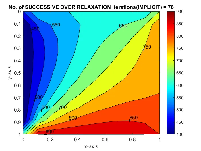
title(sprintf('No. of SUCCESSIVE OVER RELAXATION Iterations(IMPLICIT) = %d',successive_over_relaxation_iteration));
pause(0.03);

PLOT :

UNSTEADY - STATE EQUATION DISCRETIZATION :

Non-steady state situations apppear after an imposed change in temperature at a boundary as well as inside oof an object , as a result of a new source or sink of heat suddenly introducrd within an object ,causing temperature near the source or sink to change in time.

`partialT/partialt = alpha*partialT/partialx^2 + partial^T/partialy^2`

if we simplify it ,

`T_i,_j = 1/1+k1+k2*(T_i,_j+k1(T_(i-1),_j+T_(i+1,_j)+k2(T_i,_(j+1))`

JACOBI ITERATION :

 % Unsteady 2D heat conduction problem
% unsteady state condition
% iterative solver-jacobi,Gauss-seidel,Relaxation methods

clear all
close all
clc

% initial conditions
%L = 1;
nx = 10;
ny = nx;
nt = 1400;

x = linspace(0,1,nx);
y = linspace(0,1,ny);

dx = x(2)-x(1);
dy = dx;

% Abosolute error criteria > tolerance
error = 9e9;
tolerance = 1e-4;
dt = 1e-3;

% defining boundary conditions
T_L = 400;
T_T = 600;
T_R = 800;
T_B = 900;

T = 300*ones(nx,ny);

T(2:ny-1,1) = T_L;
T(2:ny-1,nx) = T_R;
T(1,2:nx-1) = T_T;
T(ny,2:nx-1) = T_B;

% calculating average temperatures at corners

T(1,1) = (T_T+T_L)/2;
T(nx,ny) = (T_R+T_B)/2;
T(1,ny) = (T_T+T_R)/2;
T(nx,1) = (T_L+T_B)/2;

% assigning  original values for T
T_old = T;
T_initial = T;


% Calculating of 2D steady heat conduction EQUATION by successive
% over-relaxattion method


k1 = 1.1*(dt/(dx^2));
k2 = 1.1*(dt/(dy^2));


jacobi_iteration = 1;

for k = 1:nt
    error = 9e9;

    while(error>tolerance)
    

    for i = 2:nx-1

        for j = 2:ny-1

            Term_1 = 1/(1+(2*k1)+(2*k2));
            Term_2 = k1*Term_1;
            Term_3 = k2*Term_1;
            H = (T_old(i-1,j))+(T_old(i+1,j));
            V = (T_old(i,j+1))+(T_old(i,j-1));

            T(i,j) = (T_initial(i,j)*Term_1)+(H*Term_2)+(V*Term_3);

        end
    end

    error = max(max(abs(T_old-T)));
    T_old = T;
    jacobi_iteration = jacobi_iteration+1;

    end

    T_initial = T;

end



% plotting
figure(1);
contourf(x,y,T,'ShowText','on');
clabel(contourf(x,y,T))
colorbar;
colormap(jet);
set(gca,'ydir','reverse')
xlabel('x-axis')
ylabel('y-axis')
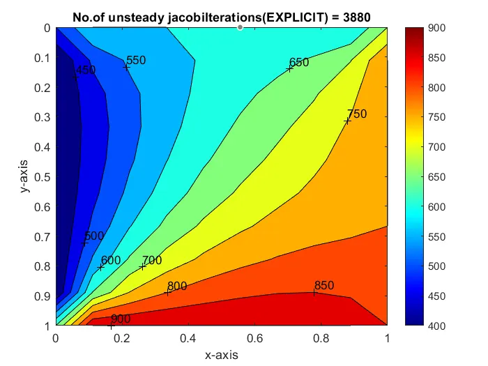
title(sprintf('No.of unsteady jacobiIterations(EXPLICIT) = %d',jacobi_iteration));
pause(0.03);

PLOT :

GAUSS-SIEDEL ITERATION :

 % Unsteady 2D heat conduction problem
% unsteady state condition
% iterative solver-jacobi,Gauss-seidel,Relaxation methods

clear all
close all
clc

% initial conditions
%L = 1;
nx = 10;
ny = nx;
nt = 1300;

x = linspace(0,1,nx);
y = linspace(0,1,ny);

dx = x(2)-x(1);
dy = dx;

% Abosolute error criteria > tolerance
error = 9e9;
tolerance = 1e-4;
dt = 1e-3;

% defining boundary conditions
T_L = 400;
T_T = 600;
T_R = 800;
T_B = 900;

T = 300*ones(nx,ny);

T(2:ny-1,1) = T_L;
T(2:ny-1,nx) = T_R;
T(1,2:nx-1) = T_T;
T(ny,2:nx-1) = T_B;

% calculating average temperatures at corners

T(1,1) = (T_T+T_L)/2;
T(nx,ny) = (T_R+T_B)/2;
T(1,ny) = (T_T+T_R)/2;
T(nx,1) = (T_L+T_B)/2;

% assigning  original values for T
T_old = T;
T_initial = T;


% Calculating of 2D steady heat conduction EQUATION by successive
% over-relaxattion method


k1 = 1.1*(dt/(dx^2));
k2 = 1.1*(dt/(dy^2));


gauss_iteration = 1;

for k = 1:nt
    error = 9e9;

    while(error>tolerance)
    

    for i = 2:nx-1

        for j = 2:ny-1

            Term_1 = 1/(1+(2*k1)+(2*k2));
            Term_2 = k1*Term_1;
            Term_3 = k2*Term_1;
            H = (T_old(i-1,j))+(T_old(i+1,j));
            V = (T_old(i,j+1))+(T_old(i,j-1));

            T(i,j) = (T_initial(i,j)*Term_1)+(H*Term_2)+(V*Term_3);

        end
    end

    error = max(max(abs(T_old-T)));
    T_old = T;
    gauss_iteration = gauss_iteration+1;

    end

    T_initial = T;

end



% plotting
figure(1);
contourf(x,y,T,'ShowText','on');
clabel(contourf(x,y,T))
colorbar;
colormap(jet);
set(gca,'ydir','reverse')
xlabel('x-axis')
ylabel('y-axis')
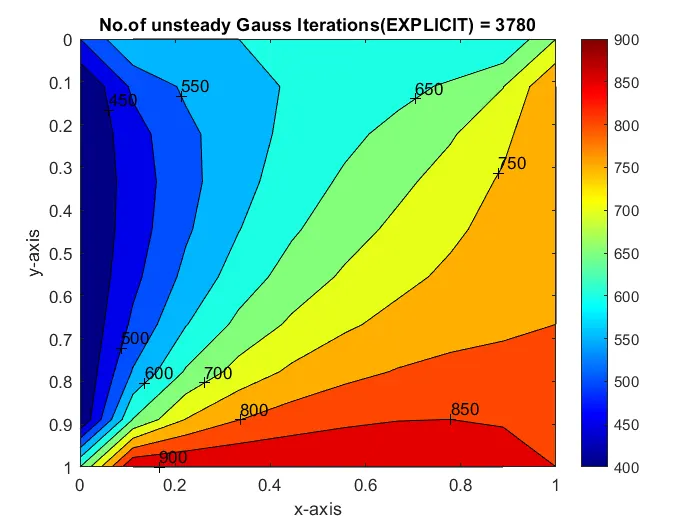
title(sprintf('No.of unsteady Gauss Iterations(EXPLICIT) = %d',gauss_iteration));
pause(0.03);

PLOT :

SUCCESSIVE - OVER RELAXATION ITERATION :

 % Unsteady 2D heat conduction problem
% unsteady state condition
% iterative solver-jacobi,Gauss-seidel,Relaxation methods

clear all
close all
clc

% initial conditions
%L = 1;
nx = 10;
ny = nx;
nt = 1400;

x = linspace(0,1,nx);
y = linspace(0,1,ny);

dx = x(2)-x(1);
dy = dx;

% Abosolute error criteria > tolerance
error = 9e9;
tolerance = 1e-4;
dt = 1e-3;
omega = 1.1;

% defining boundary conditions
T_L = 400;
T_T = 600;
T_R = 800;
T_B = 900;

T = 300*ones(nx,ny);

T(2:ny-1,1) = T_L;
T(2:ny-1,nx) = T_R;
T(1,2:nx-1) = T_T;
T(ny,2:nx-1) = T_B;

% calculating average temperatures at corners

T(1,1) = (T_T+T_L)/2;
T(nx,ny) = (T_R+T_B)/2;
T(1,ny) = (T_T+T_R)/2;
T(nx,1) = (T_L+T_B)/2;

% assigning  original values for T
T_old = T;
T_initial = T;
T_end = T;


% Calculating of 2D steady heat conduction EQUATION by successive
% over-relaxattion method

k1 = 1.1*(dt/(dx^2));
k2 = 1.1*(dt/(dy^2));


successive_over_relaxation_iteration = 1;

for k = 1:nt
    error = 9e9;

    while(error>tolerance)
    

    for i = 2:nx-1

        for j = 2:ny-1

            Term_1 = 1/(1+(2*k1)+(2*k2));
            Term_2 = k1*Term_1;
            Term_3 = k2*Term_1;
            H = (T_old(i-1,j))+(T_old(i+1,j));
            V = (T_old(i,j+1))+(T_old(i,j-1));

            T(i,j) = (T_initial(i,j)*Term_1)+(H*Term_2)+(V*Term_3);
            T_end(i,j) = ((1-omega)*T_old(i,j))+(T(i,j)*omega);

        end
    end

    error = max(max(abs(T_old-T)));
    T_old = T_end;
    successive_over_relaxation_iteration = successive_over_relaxation_iteration+1;

    end

    T_initial = T_end;

end



% plotting
figure(1);
contourf(x,y,T,'ShowText','on');
clabel(contourf(x,y,T))
colorbar;
colormap(jet);
set(gca,'ydir','reverse')
xlabel('x-axis')
ylabel('y-axis')
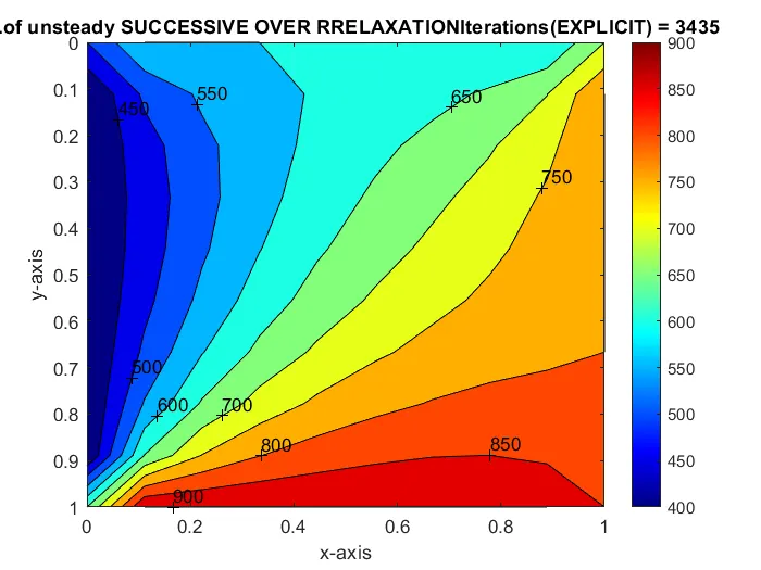
title(sprintf('No.of unsteady SUCCESSIVE OVER RRELAXATIONIterations(EXPLICIT) = %d',successive_over_relaxation_iteration));
pause(0.03);

PLOT :

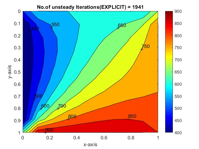
EXPLICIT SCHEME - UNSTEADY / TRANSIENT STATE CONDITION PROGRAM

UNSTEADY - STATE EQUUATION DISCRETIZATTION (EXPLICIT) :

`partial T/partialt = alpha*partial^2T/partialx^2+partial^2T/partialy^2`

if we discretize the equations it becomes,

`T_P^(n+1)-T_P^n = alpha *T_L-2T_P+T_R/partialx^2 + T_T -2T_P +T_B/partialy^2`

For the better understanding for code,

`T_i,_j =T_i,_j + k1(T_(i-1,_j)+ k2 (T_i,_(j-1 - 2T_i,_j+T_i,_(j+1))`

where ,

`k1 = alpha* trianglet/trianglex^2 , k2 = alpha *trianglet/triangley^2`

EXPLICIT SCHEME :

 % Unsteady 2D heat conduction problem
% unsteady state condition
% Explicit scheme

clear all
close all
clc

% initial conditions
%L = 1;
nx = 10;
ny = nx;
nt = 1400;

x = linspace(0,1,nx);
y = linspace(0,1,ny);

dx = x(2)-x(1);
dy = dx;

% Abosolute error criteria > tolerance
error = 9e9;
tolerance = 1e-4;
dt = 1e-3;
omega = 1.1;

% defining boundary conditions
T_L = 400;
T_T = 600;
T_R = 800;
T_B = 900;

T = 300*ones(nx,ny);

T(2:ny-1,1) = T_L;
T(2:ny-1,nx) = T_R;
T(1,2:nx-1) = T_T;
T(ny,2:nx-1) = T_B;

% calculating average temperatures at corners

T(1,1) = (T_T+T_L)/2;
T(nx,ny) = (T_R+T_B)/2;
T(1,ny) = (T_T+T_R)/2;
T(nx,1) = (T_L+T_B)/2;

% assigning  original values for T
T_initial = T;
T_old = T;



% Calculating of 2D steady heat conduction EQUATION by successive
% over-relaxattion method
iterative_solver = 1;
k1 = 1.1*(dt/(dx^2));
k2 = 1.1*(dt/(dy^2));


if iterative_solver == 1
    steady_explicit = 1;
for k = 1:nt
    error = 1;

    while(error>tolerance)
    

    for i = 2:nx-1

        for j = 2:ny-1

            Term_1 = T_old(i,j);
            Term_2 = k1*(T_old(i+1,j)-2*T_old(i,j)+(T_old(i-1,j)));
            Term_3 = k2*(T_old(i,j+1)-2*T_old(i,j)+(T_old(i,j-1)));
        
            T(i,j) = Term_1 + Term_2 + Term_3;
            

           

        end
    end

    error = max(max(abs(T_old-T)));
    T_old = T;
    steady_explicit = steady_explicit+1;

    end

end
end



% plotting
figure(1);
contourf(x,y,T,'ShowText','on');
clabel(contourf(x,y,T))
colorbar;
colormap(jet);
set(gca,'ydir','reverse')
xlabel('x-axis')
ylabel('y-axis')
title(sprintf('No.of unsteady Iterations(EXPLICIT) = %d',steady_explicit));
pause(0.03);

PLOT :

Week 5.1 - Mid term project - Solving the steady and unsteady 2D heat conduction problem

Ship work like this
in your own course.

Talk to a career counsellor

Ship work like thisin your own course.

Talk to a career counsellor

Ship work like this
in your own course.