Week 5.1 - Mid term project - Solving the steady and unsteady 2D heat conduction problem

The main aim of the project is to solve 2D-Heat conduction equation by using both implicit and explicit methods .

Here both transient and steady state equations are solved.In case of steady state only implicit methods are used and in transient state both implicit and explicit methods are used .

For both steady and unsteady state a square of unit area is considered with the below boundary conditions:

Top boundary =600K,Bottom boundary =900K, Left boundary =400K and right boundary = 800K.

1)Steady state: In steady state the variables at a point does not change with time.

The steady state heat conduction equation is

`(del^2T)/(delx^2)+(del^2T)/(dely^2)=0`------------------------(1)

since equation 1 is elliptic in nature it requires the data or information from all the directions so a central scheme is used for discretization.

after discretization the eqaution obtained is shown below:

`T(i,j)=1/k((T(i-1,j)+T(i+1,j))/(△x^2)+(T(i,j+1)+T(i,j-1))/(△y^2))`------------------2

k=`(2*(△x^2+△y^2))/(△x^2*△y^2)`

Since we are using implicit method of discretization we need to use iterative solvers to solve equation(2)

In this project point interative techniques are used :

a)Jacobi method

b)Gauss Siedel method

c)Sucessive over relaxation method

The steady state equation is solved by using 3 techniques for the same conditions so that it enables us to compare them.

The entire project is carried out on MATlab.

The code used is explained and shown below :

clear all 
close all 
clc 

%initial cnditions 
nx=10;
ny=nx;
x=linspace(0,1,nx);  %mesh 
y=linspace(0,1,ny);
dx=x(2)-x(1);
dy=dx;

T=300*ones(nx,ny);

%boundary conditions 
T(1,:)=600;  %top bc
T(nx,:)=900;  %bottom bc
T(:,1)=400; % left bc
T(:,ny)=800;  %right bc 

% edge bc are obtained by taking average between 2 surfaces 

T(1,1)=500;
T(nx,1)=650;
T(1,ny)=700;
T(nx,ny)=850;

Told=T;

error=9e9;
tolerance=1e-4;
k=2*((dx^2+dy^2)/(dx^2*dy^2));

iterative_solver=input('Enter : 1-for jacobi, 2- for gauss siedal,3-for Sucessive over relaxation = ');

if(iterative_solver==1)  %jacobi
   tic
    jacobi_iter=1;
    
    while(error>tolerance)
        
        for i=2:nx-1
            for j=2:ny-1
                
                T(i,j)=((Told(i-1,j)+Told(i+1,j))/(dx^2)+(Told(i,j+1)+Told(i,j-1))/(dy^2))/k;
            end
        end
        error=max(max(abs(Told-T)));
        Told=T;
        jacobi_iter=jacobi_iter+1;
        
        %plotting contour 
        figure(1)
       contourf(x,y,T)
       clabel(contourf(x,y,T))
       colorbar
       colormap(jet)
       set(gca,'ydir','reverse')
       xlabel('X-axis')
       ylabel('Y-axis')
       title_text=sprintf('No of Jacobi iterations =%d',jacobi_iter);
       title(title_text);
       pause(0.03)
      
    end
    time_taken_for_simulation_jacobi=toc
end

if(iterative_solver==2) % gauss siedal 
       
    tic
    gauss_iter=1;
    
    while(error>tolerance)
        
        for i=2:nx-1
            for j=2:ny-1
                
                T(i,j)=((T(i-1,j)+Told(i+1,j))/(dx^2)+(Told(i,j+1)+T(i,j-1))/(dy^2))/k;
            end
        end
        error=max(max(abs(Told-T)));
        Told=T;
        gauss_iter=gauss_iter+1;
        
        %plotting contour 
        figure(1)
       contourf(x,y,T)
       clabel(contourf(x,y,T))
       colorbar
       colormap(jet)
       set(gca,'ydir','reverse')
       xlabel('X-axis')
       ylabel('Y-axis')
       title_text=sprintf('No of Gauss Siedal iterations =%d',gauss_iter);
       title(title_text);
       pause(0.03)
      
    end
    time_taken_for_simulation_Gauss=toc
end

if(iterative_solver==3) % sucessive over relaxation 
    tic
    sor_iter=1;
    omega=1.3;
    
    while(error>tolerance)
        
        for i=2:nx-1
            for j=2:ny-1
                
                T(i,j)=(1-omega)*Told(i,j)+omega*((T(i-1,j)+Told(i+1,j))/(dx^2)+(Told(i,j+1)+T(i,j-1))/(dy^2))/k;
            end
        end
        error=max(max(abs(Told-T)));
        Told=T;
        sor_iter=sor_iter+1;
        
        %plotting contour 
        figure(1)
       contourf(x,y,T)
       clabel(contourf(x,y,T))
       colorbar
       colormap(jet)
       set(gca,'ydir','reverse')
       xlabel('X-axis')
       ylabel('Y-axis')
       title_text=sprintf('No of SOR iterations =%d',sor_iter);
       title(title_text);
       pause(0.03)
      
    end
    time_taken_for_simulation_SOR=toc
end
 

Explanation of code:

• The first step is intializing the conditions which are nothing but defining number of nodes in x and y direction.
• Mesh is generated by using linspace command .
• Since we are using iterative techniques we need to provide a guess value whic is defined as T=300*ones(nx,ny).
• Next step is incorporating the boundary conditions.
• In the begining the error value is assumed to be 9e9 and tolearnce which is required for convergence of the solution is 1e-4.
• Since we have 3 techniques an if command is utilized to select between these 3 techniques.
• For all the 3 techniques the loop structure is same only the equation(2) is modifed according to the method .
• The basic iterative structure consists of 2 loops those are :
• 1)while loop which is nothing but the convergence loop which repeates the calculation till our error term is less than tolerance.
• 2) Space loop which is used for calculating the variation of variables in space . since we dealing with 2 dimensions 2 for loops are used .
• These for loops are varying from 2 to nx-1 or ny-1 because central scheme is incoprated in discretization.
• After the for loops the error term is calculated and the old values are updated.
• The above mentioned structure remains the same for all the 3 methods but the equations (2) changes .
• For the jacobi method the equation (2) uses only the old values in calculating the next step values.
• For the Gauss siedel method the equation(2) uses the updated values for calculating the nextstpe values.
• In Sucessive over relaxation method a term omega is introduced to either jacobi or Gauss siedel method so get the convergence faster.
• The final step involves plotting the variation of tempearture this done by using the contour command as shown above.

Outputs and results (Steady state):

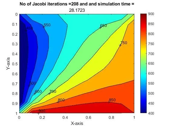
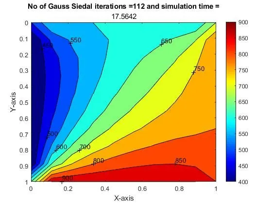
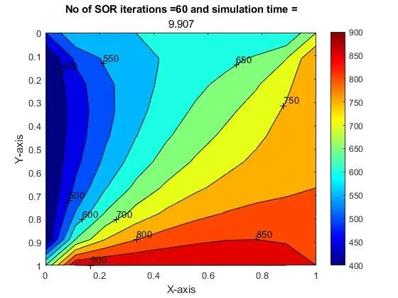
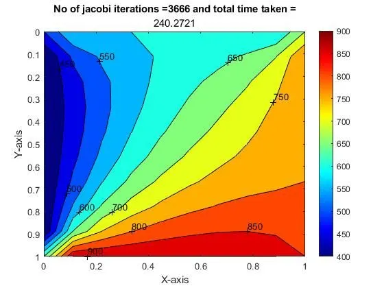
The contours , number of iterations and siumlation time taken for all the methods are shown below :

a) Jacobi method:

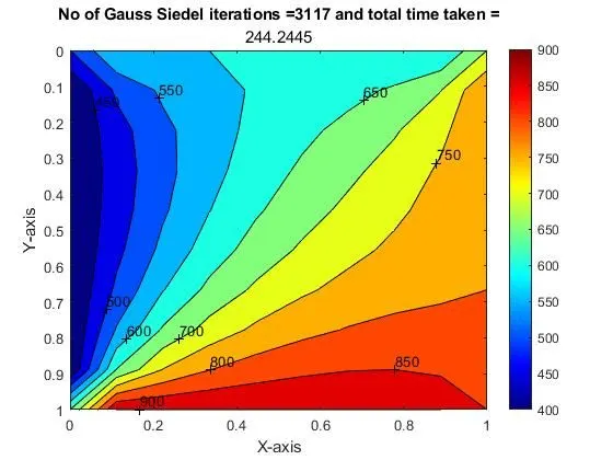
b)Gauss Siedel :

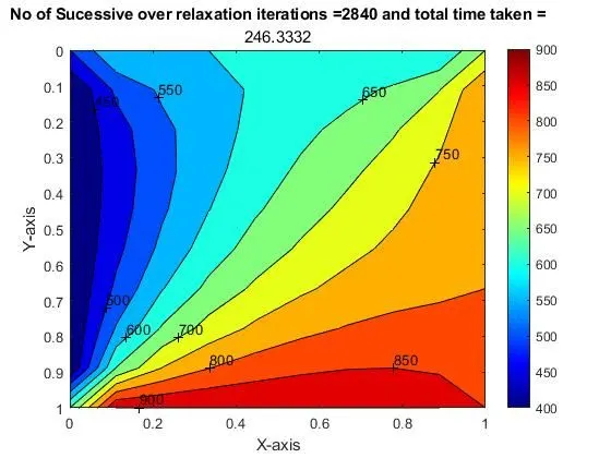
c) Sucessive over relaxation :

Results and conclusion (steady state):

• It is clearly observed from the above figures that the number of iterations required for the solution to converge is lowest in case of Sucessive over relaxation method follwed by Gauss Siedel and Jacobi method.
• Since the no of iterations to converge is less in case of SOR method obviously the simuation time taken will also be less compared to other methods .

2) Trasnient state analysis :

The transient heat equation is

`(delT)/(delt)=(del^2T)/(delx^2)+(del^2T)/(dely^2)`--------------------(3)

Forward difference in time and central difference in space is used for discretization.

After discretization the eqaution 3 becomes

`overset(n+1)(T(i,j))=overset(n)(T(i,j))+alpha△T*((T(i-1,j)-2*T(i,j)+T(i+1,j))/(△x^2)+(T(i,j-1)-2*T(i,j)+T(i,j+1))/(△y^2))^n`-----(4)

Equation 4 is for explict.

`overset(n+1)(T(i,j))=overset(n)(T(i,j))+alpha△T*((T(i-1,j)-2*T(i,j)+T(i+1,j))/(△x^2)+(T(i,j-1)-2*T(i,j)+T(i,j+1))/(△y^2))^(n+1)`-----(5)`

Equation 5 is implicit because the RHS is taken at next step ie n+1.

The transient state analysis is performed by using both implicit and explicit methods .

Solving transient heat eqaution by using explicit method:

The code used is explained and shown below:

clear all 
close all 
clc 

%initial cnditions 
nx=10;
ny=nx;
x=linspace(0,1,nx);  %mesh 
y=linspace(0,1,ny);
dx=x(2)-x(1);
dy=dx;
dt=1e-3; 
nt=1400; %no of time steps  

%total simlation run time = nt*n=1400*0.001=1.4 seconds 

T=ones(nx,ny);

%boundary conditions 
T(1,:)=600;  %top bc
T(nx,:)=900;  %bottom bc
T(:,1)=400; % left bc
T(:,ny)=800;  %right bc 

% edge bc are obtained by taking average between 2 surfaces 

T(1,1)=500;
T(nx,1)=650;
T(1,ny)=700;
T(nx,ny)=850;

Told=T;
alpha=1.4; % thermal conductivity 

k1=alpha*(dt/dx^2); %cfl number in x 
k2=alpha*(dt/dy^2);  %cfl number in y 
%for stability k1+k2 <= 0.5 
CFL=k1+k2;

%in this program the transient heat conduction is solved by using explicit

%time loop 
tic
iter=1;
for k=1:nt 
    
    for i=2:nx-1  %space loop 
        
        for j=2:ny-1
            
            T(i,j)=Told(i,j)+k1*(Told(i-1,j)-2*(Told(i,j))+Told(i+1,j))+k2*(Told(i,j+1)-2*(Told(i,j))+Told(i,j-1));
            
        end
    end
    Told=T;
    iter=iter+1;
    
    %plotting 
    
    figure(1)
    contour(x,y,T)
    clabel(contourf(x,y,T))
    colorbar
    colormap(jet)
    set(gca,'ydir','reverse')
    xlabel('X-axis')
    ylabel('Y-axis')
    title_text=sprintf('No of jacobi iterations =%d',iter);
    title(title_text);
    pause(0.3)
    
end
time_taken_for_simulation=toc

Explanation of the code :

• The first step is intializing the conditions which are nothing but defining number of nodes in x and y direction.
• The second step is specifying the number of time steps and size of each time step . Here the utmost care has to be taken because we need to choose values of nt and dt in such a way that the there is stability and also giving enough timesteps for the simulation so that a steady state is achieved.
• Next step is prvinding the values of alpha which is thermal conductivity of the material which is choosen to be 1.4 .
• Mesh is generated by using linspace command .
• Next step is incorporating the boundary conditions.
• Since we are using explicit method the soluition is straight forward and in this technique there is no requirement of iterative solvers.
• The basic structure consists of 2 loops those are :
• 1)Time loop which is nothing but a loop which repeates the calculation for every single time step because we dealing with transient condtions the variables changes with time.
• 2) Space loop which is used for calculating the variation of variables in space . since we dealing with 2 dimensions 2 for loops are used .
• These for loops are varying from 2 to nx-1 or ny-1 because central scheme is incoprated in discretization.
• After the old values are updated.
• The final step involves plotting the variation of tempearture this done by using the contour command as shown above.

Output and results :

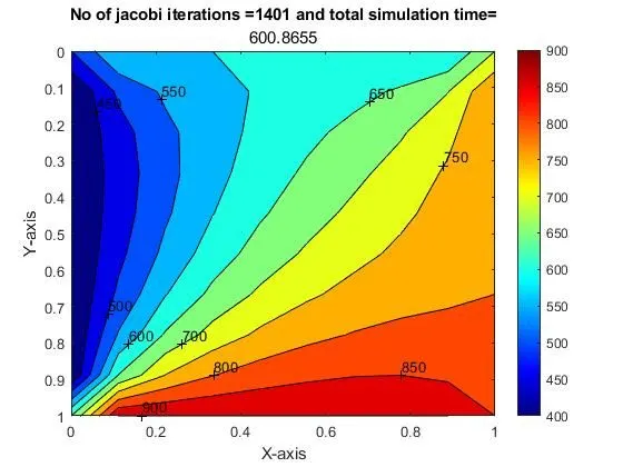
The contour, number of iterations and siumlation time taken are shown below :

Output (tansient explicit) :

Solving Transient heat equation by using implicit method :

The transient heat equation is solved by using 3 methods :

a)Jacobi method

b)Gauss Siedel method

c)Sucessive over relaxation method

The code used is explained and shown below:

clear all 
close all 
clc 

%initial cnditions 
nx=10;
ny=nx;
x=linspace(0,1,nx);  %mesh 
y=linspace(0,1,ny);
dx=x(2)-x(1);
dy=dx;
dt=1e-3; 
nt=1400; %no of time steps  

tolerance=1e-4;


%total simlation run time = nt*n=1400*0.001=1.4 seconds 

T=300*ones(nx,ny);

%boundary conditions 
T(1,:)=600;  %top bc
T(nx,:)=900;  %bottom bc
T(:,1)=400; % left bc
T(:,ny)=800;  %right bc 

% edge bc are obtained by taking average between 2 surfaces 

T(1,1)=500;
T(nx,1)=650;
T(1,ny)=700;
T(nx,ny)=850;

Told=T;
Tprev=Told;

alpha=1.4; % thermal conductivity 

k1=alpha*(dt/dx^2); %cfl number in x 
k2=alpha*(dt/dy^2);  %cfl number in y 


%in this program the transient heat conduction is solved by using explicit
%jacobi method
iterative_solver=input('Enter : 1-for jacobi, 2- for gauss siedal,3-for Sucessive over relaxation = ');

if(iterative_solver==1)

tic
jacobi_iter=1;
for k=1:nt 
    error=9e9;
    while(error>tolerance)
    
    for i=2:nx-1
        
        for j=2:ny-1
            
            T(i,j)=(Tprev(i,j)+k1*(Told(i-1,j)+Told(i+1,j))+k2*(Told(i,j+1)+Told(i,j-1)))/(1+2*k1+2*k2);
            
        end
    end
    error=max(max(abs(Told-T)));
    Told=T;
    jacobi_iter=jacobi_iter+1;
    
    end
    Tprev=T;
    figure(1)
    contour(x,y,T)
    clabel(contourf(x,y,T))
    colorbar
    colormap(jet)
    set(gca,'ydir','reverse')
    xlabel('X-axis')
    ylabel('Y-axis')
    title_text=sprintf('No of jacobi iterations =%d',jacobi_iter);
    title(title_text);
    pause(0.03)
    
end

time_taken_for_simulation_jacobi=toc

end

if(iterative_solver==2) %gauss siedel 

tic
gs_iter=1;
for k=1:nt 
    error=9e9;
    while(error>tolerance)
    
    for i=2:nx-1
        
        for j=2:ny-1
            
            T(i,j)=(Tprev(i,j)+k1*(T(i-1,j)+Told(i+1,j))+k2*(Told(i,j+1)+T(i,j-1)))/(1+2*k1+2*k2);
            
        end
    end
    error=max(max(abs(Told-T)));
    Told=T;
    gs_iter=gs_iter+1;
    
    end
    Tprev=T;
    figure(1)
    contour(x,y,T)
    clabel(contourf(x,y,T))
    colorbar
    colormap(jet)
    set(gca,'ydir','reverse')
    xlabel('X-axis')
    ylabel('Y-axis')
    title_text=sprintf('No of Gauss Siedel iterations =%d',gs_iter);
    title(title_text);
    pause(0.03)
    
end

time_taken_for_simulation_gauss_siedel=toc

end


if(iterative_solver==3) %Sucessive over relaxation 

tic
sor_iter=1;
for k=1:nt 
    error=9e9;
    omega=1.3;
    while(error>tolerance)
    
    for i=2:nx-1
        
        for j=2:ny-1
            
            T(i,j)=(1-omega)*Tprev(i,j)+omega*(Tprev(i,j)+k1*(T(i-1,j)+Told(i+1,j))+k2*(Told(i,j+1)+T(i,j-1)))/(1+2*k1+2*k2);
            
        end
    end
    error=max(max(abs(Told-T)));
    Told=T;
    sor_iter=sor_iter+1;
    
    end
    Tprev=T;
    figure(1)
    contour(x,y,T)
    clabel(contourf(x,y,T))
    colorbar
    colormap(jet)
    set(gca,'ydir','reverse')
    xlabel('X-axis')
    ylabel('Y-axis')
    title_text=sprintf('No of Sucessive over relaxation iterations =%d',sor_iter);
    title(title_text);
    pause(0.03)
    
end

time_taken_for_simulation_SOR=toc

end

Explanation of the code :

• The first step is intializing the conditions which are nothing but defining number of nodes in x and y direction.
• Mesh is generated by using linspace command .
• The second step is specifying the number of time steps and size of each time step .
• Next step is prvinding the values of alpha which is thermal conductivity of the material which is choosen to be 1.4 .
• Since we are using iterative techniques we need to provide a guess value whic is defined as T=300*ones(nx,ny).
• Next step is incorporating the boundary conditions.
• In the begining the error value is assumed to be 9e9 and tolearnce which is required for convergence of the solution is 1e-4.
• Since we have 3 techniques an if command is utilized to select between these 3 techniques.
• For all the 3 techniques the loop structure is same only the equation(5) is modifed according to the method .
• The basic iterative structure consists of 3 loops those are :
• 1)Time loop which is nothing but a loop which repeates the calculation for every single time step because we dealing with transient condtions the variables changes with time.
• 2)while loop which is nothing but the convergence loop which repeates the calculation till our error term is less than tolerance.
• 3) Space loop which is used for calculating the variation of variables in space . since we dealing with 2 dimensions 2 for loops are used .
• These for loops are varying from 2 to nx-1 or ny-1 because central scheme is incoprated in discretization.
• After the for loops the error term is calculated and the old values are updated.
• The above mentioned structure remains the same for all the 3 methods but the equations (5) changes .
• For the jacobi method the equation (5) uses only the old values in calculating the next step values.
• For the Gauss siedel method the equation(5) uses the updated values for calculating the nextstpe values.
• In Sucessive over relaxation method a term omega is introduced to either jacobi or Gauss siedel method so get the convergence faster.
• The final step involves plotting the variation of tempearture this done by using the contour command as shown above.

Outputs(Treansient implicit ):

The contours , number of iterations and siumlation time taken for all the methods are shown below .

a)Jacobi method output:

b)Gauss Siedel method :

c)Sucessive over relaxation method:

Result(Transient implicit method):

• It is clearly observed from the above figures that the number of iterations required for the solution to converge is lowest in case of Sucessive over relaxation method follwed by Gauss Siedel and Jacobi method.

Results and conclusion (Transient analaysis for both implicit and explicit)

• On comparing both the methods the amount of time taken for simuation is considerably high for an explicit method and number of iterations is considerably more for implicit method.