Week 3.5 - Deriving 4th order approximation of a 2nd order derivative using Taylor Table method

This challenge has 2 parts ,the first part consists of findiing out the fourth order approximation of a second order derviative by using central scheme, skewed right sided difference and by skewed left sided difference .The technique used in finding the approximation is Taylor's table method.

The second part of the challenge is to apply the derived approximation on a function f(x)=`exp(x)*cosx`and to compare it with the exact solution to visualize the error variations. The second part of this challenge is completely performed on MATLAB.

First part of the challenge :

a)cental difference scheme:

To start with the taylors table method we need to know the stencil size for that a simple formula is used:

order of approximation = number of nodes in stencil -order of derivative +1

4=n-2+1

n=5 ie no nodes in stencil for central scheme.

let the approximation of a 2nd order dervative of a function be `(del^2f)/(delx^2)=af(i-2)+bf(i-1)+cf(i)+df(i+1)+ef(i+2)`........................(1)

taylors table : The expansion of each term in the stencil is arranged in talors table

	f(i)	`f'(i)(dx)`	`f''(i)(dx^2)`	`f'''(i)(dx^3)`	`f''''(i)(dx^4)`	`f'''''(i)(dx^5)`	`f''''''(i)(dx^6)`
a*f(i-2)	a	-2a	4a/2	-8a/6	+16a/24	-32a/120	64a/240
b*f(i-1)	b	-b	b/2	-b/6	b/24	-b/120	b/240
c*f(i)	c	0	0	0	0	0	0
d*f(i+1)	d	d	d/2	d/6	d/24	d/120	d/240
e*f(i+2)	e	2e	4e/2	8e/6	16e/24	32e/120	64e/240
`(del^2f)/(delx^2)=sum` of all above terms	0	0	1	0	0	??????	???????

We are finding out the approximation for 2nd order derivative so the sum of column 4 is equated for 1 and rest all to zero since we need 5 equations to solve for five unknowns the last 2 columns is unknown for us and also because our stencil consists of only 5 terms I can only perdict for the first 5 terms in expansion rest all simply we dont know.

Then we have 5 equations with 5 unknowns:

a+b+c+d+e=0

-2a+-b+d+2e=0

4a/2+b/2+d/2+de/2=1

-8a/6-b/6+d/6+8e/6=0

2a/3+b/24+d/24+2e/3=0

solving the above equations by using matrices

`[[1,1,1,1,1],[-2,-1,0,1,2],[4/2,1/2,0,1/2,4/2],[-8/6,-1/6,0,1/6,8/6],[2/3,1/24,0,1/24,2/3]][[a],[b],[c],[d],[e]]=[[0],[0],[1],[0],[0]]`.

AX=B

X=A'B

after solving the vaules are:

a=-0.083333

b=1.333333

c=-2.500000

d=1.333333

e=-0.083333

sum of coefficients of column 2,3,5and 6 are zero

sum of coefficients of column 4 is 1

sum of coefficients of column 4 and 7 are non-zero

therefore the remaning terms in column 4 is to the power `(dx)^2`and for column 7 is `(dx)^6`

so therefore divindng the equation (1) by (dx)^2 ;

then eqaution 1 becomes: `(del^2f)/(delx^2)=(af(i-2)+bf(i-1)+cf(i)+df(i+1)+ef(i+2))/(dx)^2+f''''''(i) (△x)^4`

by doing this the remaning term in the expanision is (dx)^4 ,therfore fourth order approximation.

b) skewed right side difference:

To start with the taylors table method we need to know the stencil size for that a simple formula is used:

order of approximation = number of nodes in stencil -order of derivative

4=n-2

n=6 ie no nodes in stencil for skewed right side difference scheme.

let the approximation of a 2nd order dervative of a function be `(del^2f)/(delx^2)=af(i)+bf(i+1)+cf(i+2)+df(i+3)+ef(i+4)+gf(i+5)`........................(2)

taylors table : The expansion of each term in the stencil is arranged in talors table

	f(i)	`f'(i)(dx)`	`f''(i)(dx^2)`	`f'''(i)(dx^3)`	`f''''(i)(dx^4)`	`f'''''(i)(dx^5)`	`f''''''(i)(dx^6)`
a*f(i)	a	0	0	0	0	0	0
b*f(i+1)	b	b	b/2	b/6	b/24	b/120	b/720
c*f(i+2)	c	2c	4c/2	8c/6	16c/24	32c/120	64c/720
d*f(i+3)	d	3d	9d/2	27d/6	81d/24	243d/120	729d/720
e*f(i+4)	e	4e	16e/2	64e/6	256e/24	1024e/120	4096e/720
g*f(i+5)	g	5g	25g/2	125g/6	625g/24	3125g/120	15625g/720
`(del^2f)/(delx^2)=sum` of all above terms	0	0	1	0	0	0	???????

We are finding out the approximation for 2nd order derivative so the sum of column 4 is equated for 1 and rest all to zero since we need 6 equations to solve for six unknowns the last column is unknown for us and also because our stencil consists of only 6 terms I can only perdict for the first 6 terms in expansion rest all simply we dont know.

Then we have 6 equations with 6 unknowns:

a+b+c+d+e+g=0

0+b+2c+3d+de+5g=0

0+b/2+2c+9d/2+8e+25g/2=1

0+b/6+8c/6+27d/6+64e/6+125g/6=0

0+b/24+16c/24+81d/24+256e/24+625g/24=0

0+b/120+32c/120+243d/120+1024e/120+3125g/120=0

solving the above equations by using matrices

`[[1,1,1,1,1,1],[0,1,2,3,4,5],[0,1/2,2,9/2,8,25/2],[0,1/6,8/6,27/6,64/6,125/6],[0,1/24,16/24,81/24,256/24,1024/120],[0,1/120,32/120,243/120,1024/120,3125/120]][[a],[b],[c],[d],[e],[g]]=[[0],[0],[1],[0],[0],[0]]``

AX=B

X=A'B

after solving the vaules are:

a=3.750000

b=-12.833333

c=17.833333

d=-13.000000

e=5.083333

g=-0.833333

sum of coefficients of column 2,3,5and 6 are zero

sum of coefficients of column 4 is 1

sum of coefficients of column 4 and 7 are non-zero

therefore the remaning terms in column 4 are to the power `(dx)^2`and for column 7 is `(dx)^6`

so therefore divindng the equation (2) by (dx)^2 ;

then equation 2 becomes

`(del^2f)/(delx^2)=(af(i)+bf(i+1)+cf(i+2)+df(i+3)+ef(i+4)+gf(i+5))/(dx^2)+f''''''(i) (△x)^4`

by doing this the highest term in the remaning expanision is (dx)^4 ,therfore fourth order approximation.

c)skewed left side difference:

To start with the taylors table method we need to know the stencil size for that a simple formula is used:

order of approximation = number of nodes in stencil -order of derivative

4=n-2

n=6 ie no nodes in stencil for skewed left side difference scheme.

let the approximation of a 2nd order dervative of a function be `(del^2f)/(delx^2)=af(i-5)+bf(i-4)+cf(i-3)+df(i-2)+ef(i-1)+gf(i)`........................(3)`

taylors table : The expansion of each term in the stencil is arranged in talors table

	f(i)	`f'(i)(dx)`	`f''(i)(dx^2)`	`f'''(i)(dx^3)`	`f''''(i)(dx^4)`	`f'''''(i)(dx^5)`	`f''''''(i)(dx^6)`
a*f(i-5)	a	-5a	25a/2	-125a/6	625a/24	-3125a/120	15625a/720
b*f(i-4)	b	-4b	8b	-64b/6	256b/24	-1024b/120	4096b/720
c*f(i-3)	c	-3c	9c/2	-27c/6	81c/24	-243c/120	729c/120
d*f(i-2)	d	-2d	2d	-8d/6	16d/24	-32d/120	64d/720
e*f(i-1)	e	-e	e/2	-e/6	e/24	-e/120	e/720
g*f(i)	g	0	0	0	0	0	0
`(del^2f)/(delx^2)=sum` of all above terms	0	0	1	0	0	0	???????

We are finding out the approximation for 2nd order derivative so the sum of column 4 is equated for 1 and rest all to zero since we need 6 equations to solve for six unknowns the last column is unknown for us and also because our stencil consists of only 6 terms I can only perdict for the first 6 terms in expansion rest all simply we dont know.

Then we have 6 equations with 6 unknowns:

a+b+c+d+e+g=0

-5a-4b-3c-2d-e+0=0

25a/2+8b+9c/2+2d+e/2+0=1

-125a/6-64b/6-27c/6-8d/6-e/6+0=0

625a/24+256b/24+81c/24+16d/24+e/24+0=0

-3125a/120-1024b/120-243c/120-32d/120-e/120+0=0

solving the above equations by using matrices

`[[1,1,1,1,1,1],[-5,-4,-3,-2,-1,0],[25/2,8/2,9/2,2,1/2,0],[-125/6,-64/6,-27/6,-8/6,-1/6,0],[625/24,256/24,81/24,16/24,1/24,0],[-3125/120,-1024/120,-243/120,-32/120,-1/120,0]][[a],[b],[c],[d],[e],[g]]=[[0],[0],[1],[0],[0],[0]]`

AX=B

X=A'B

after solving the vaules are:

a=-0.833333

b=5.083333

c=-13.000000

d=17.833333

e=-12.833333

g=3.750000

sum of coefficients of column 2,3,5and 6 are zero

sum of coefficients of column 4 is 1

sum of coefficients of column 4 and 7 are non-zero

therefore the remaning terms in column 4 are to the power `(dx)^2`and for column 7 is `(dx)^6`

so therefore divindng the equation (3) by (dx)^2 ;

then equation 3 becomes

`(del^2f)/(delx^2)=(af(i-5)+bf(i-4)+cf(i-3)+df(i-2)+ef(i-1)+gf(i))/(dx^2)+f''''''(△x)^4`.

Second part of the challenge:

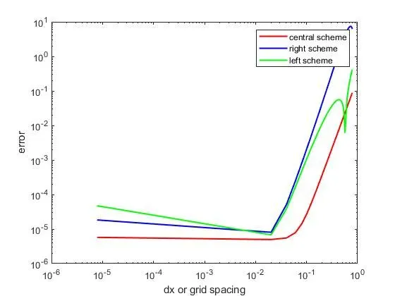
For the second part of the challenge the second order derivative of the function f(x)=exp(x)*cos(x) is calculated exactly and also by using fourth order approximate central , left skewed and right skewed schemes and grid spacing (dx) v/s error term is plotted to visulize how the error is varying for 3 different schemes.

The exact second order derivative of the function f(x) is

`f''(x)=-2exp(x)*sin(x)`

The calculation of second order derivatice is done at x=pi/3 and for dx varying from pi/400000 to pi/4.

The entire calculation is performed on MATLAB. The code which is used is shown below and explained parallely:

The code can be explained in 3 parts:

partx: Creation of respective functions to get error term.

function#1- For central difference scheme fourth order approximation.

function cd_error=cd_fourth_order(x,dx)

exact_solution=-2*exp(x)*sin(x);

a=-0.083333;
b=1.333333;
c=-2.500000;
d=1.333333;
e=-0.083333;

f1=exp(x-2*dx)*cos(x-2*dx);
f2=exp(x-dx)*cos(x-dx);
f3=exp(x)*cos(x);
f4=exp(x+dx)*cos(x+dx);
f5=exp(x+2*dx)*cos(x+2*dx);

central_difference=((a*f1)+(b*f2)+(c*f3)+(d*f4)+(e*f5))/(dx^2);

cd_error=abs(exact_solution-central_difference);


end

Function#2-For right skewed scheme

% for right skewed 
function error=srsd_fourth_order(x,dx)

exact_solution=-2*exp(x)*sin(x);

a=3.750000;
b=-12.833333;
c=17.833333;
d=-13.000000;
e=5.083333;
g=-0.833333;

f1=exp(x)*cos(x);
f2=exp(x+dx)*cos(x+dx);
f3=exp(x+2*dx)*cos(x+2*dx);
f4=exp(x+3*dx)*cos(x+3*dx);
f5=exp(x+4*dx)*cos(x+4*dx);
f6=exp(x+5*dx)*cos(x+5*dx);

right_skewed_diff=((a*f1)+(b*f2)+(c*f3)+(d*f4)+(e*f5)+(g*f6))/(dx^2);

error=abs(right_skewed_diff-exact_solution);


end

Function#3-For left skewed scheme:

%for left skewed approximation

function error=slsd_fourth_order(x,dx)

exact_solution=-2*exp(x)*sin(x);

a=-0.833333;
b=5.083333;
c=-13.000000;
d=17.833333;
e=-12.833333;
g=3.750000;

f1=exp(x-5*dx)*cos(x-5*dx);
f2=exp(x-4*dx)*cos(x-4*dx);
f3=exp(x-3*dx)*cos(x-3*dx);
f4=exp(x-2*dx)*cos(x-2*dx);
f5=exp(x-dx)*cos(x-dx);
f6=exp(x)*cos(x);

left_skewed_diff=((a*f1)+(b*f2)+(c*f3)+(d*f4)+(e*f5)+(g*f6))/(dx^2);

error=abs(left_skewed_diff-exact_solution);


end

Part y: In this part the error term is calculated for range of dx by creating a for loop and calling the repective functions.

close all
clear all
clc

x=pi/3;

dx=linspace(pi/40000,pi/4,40);

for i=1:length(dx)
    
   centre_scheme(i)=cd_fourth_order(x,dx(i));
   right_scheme(i)=srsd_fourth_order(x,dx(i));
   left_scheme(i)=slsd_fourth_order(x,dx(i));   
    
end


%plotting graph


figure(1)

loglog(dx,centre_scheme,'r','linewidth',1.5)
hold on
loglog(dx,right_scheme,'b','linewidth',1.5)
hold on
loglog(dx,left_scheme,'g','linewidth',1.5)

xlabel('dx or grid spacing')
ylabel('error')
legend('central scheme','right scheme','left scheme')

Part z: This part involves plotting graph betwwen grid spacing (dx) and error term for various schemes to visulaize how the error is changing.

Outputs:

The output of the program is the graph which shows the variation of error for various schemes with respect to grid spacing(dx).

Conclusion:

1) For all the 3 schemes the error term decreases with decrease in grid spacing value .In between these three the central scheme has the lowest error compared to skewed schemes.

The error term decreases only till a certain point , why ???

After a certain range of dx it is clearly observed from the graph that the error value is graduly increasing this is because the round off error is dominating the truncation error . This situation can be tackled by inputting the coefficients in fraction format.

2) What is the requirement for skewed scheme when central scheme has lowest error???

If you observe the hypothetical functions for all the schemes (ie eq 1,2,3),the central scheme uses information from both the sides of the stencil to calculate the value at a point whereas the skewed schemes utliztes the information only from either left or from right side . This might be advantageous in some situation where we have information on only one side of the problem or Suppose when we are trying find the values at the boundaries skewed scheme provides a soltion .

So in some the cases even if the error produced by central scheme is low we cannot apply it , so in those kinds of situation skewed schemes are helpful.