Week 5.1 - Mid term project - Solving the steady and unsteady 2D heat conduction problem
Aim : is to solve the steady and unsteady heat conduction equation by using iterative solvers like jacobi,gauss seidel,succesive over relaxation method.
Objective :
is to solve Steady state analysis & Transient State Analysis
Solve the 2D heat conduction equation by using the point iterative techniques .
a) The Boundary conditions for the problem is given below
because of the 2d equation we have the two directions named as x & y.the total no of nodes we assume on both the directions is 10. so that we have taken nx=ny=10;
- Top Boundary = 600 K
- Bottom Boundary = 900 K
- Left Boundary = 400 K
- Right Boundary = 800 K
- along with the boundary conditions, we have taken 300k of initial temperature at all the other nodes
have to implement the following methods for solving implicit equations.
- Jacobi
- Gauss-seidel
- Successive over-relaxation
given absolute error criteria is 1e-4
b) to write code for both implicit and explicit schemes (This is for the Transient Analysis only)
c) to Write a detailed explanation for your results, plots or codes
steady state analysis of 2D heat conduction equation :
If the temperature of a body does not vary with time, it is said to be in steady state
2D heat conduction equation for steady state :
`(partial^2u)/(partialx^2)+(partial^2u)/(partialy^2)=0`
since it is 2d equation it has we may know it presents 2 axises with 4 quardrants.
here we are denoted those axises are in the form of indices those are i.j,so that it wouldbe easy to understand.
Elliptical Equation
The characteristics curve for Elliptical Equation are imaginary. We don’t have limited region of influence or domain of dependence, rather information is propagated everywhere in all directions. This is the major characteristics of Elliptical equation. Let us consider a closed domain abcd as shown in above picture, If we introduce a disturbance at point P, the disturbance will be felt everywhere throughout the domain. Therefore solution at point P has to be computed simultaneously with the solution of all other points in the domain abcd. Such solution approach is totally different from the “marching approach” of parabolic and hyperbolic equations. We need to specify boundary condition for all boundaries in the computational domain. These boundary condition can be Dirichlet or Newmann or Mixed type. So this is a Boundary-Value Problem.
Steady Inviscid Subsonic Flow are governed by Elliptical Equation. Steady Euler Equations for Mach number less than 1 are Elliptical in Nature. In subsonic flow, disturbance propagates faster than the source and it propagates to infinity in all directions. Such is the pattern of streamline for subsonic flow over aerofoil as shown above. Notice that Streamlines in front of aerofoil deflected upward and behind the aerofoil deflected downward. Disturbance introduced by the presence of aerofoil are felt throughout the entire flow field. Above picture is a picture consistent with the mathematical behavior of elliptical equation.
Steady state conduction is an example of Elliptical equation. In the elliptical equation disturbance propagates in all directions at infinite speed. Solution in domain always smooth/continuous because disturbance propagates in all directions at infinite speed. (Boundary value problem) Boundary can have discontinuities so the effect of discontinuities from the boundary dissipates very rapidly & Disturbance felt and dissipates rapidly in the entire domain.
since the present temperature of this equation is always depends on the all the other neighbouring temperature values so that we are going to use 2nd order central difference approximation method to sole the equation.
`implies(partial^2u)/(partialx^2)+(partial^2u)/(partialy^2)=0`
steady state equation descritization :
`implies(T_(i+1,j)-2T_(i,j)+T_(i-1,j))/(Deltax^2)+(T_(i,j+1)-2T_(i,j)+T_(i,j-1))/(Deltay^2)=0`
`implies(T_(i+1,j)+T_(i-1,j))/(Deltax^2)+(T_(i,j+1)+T_(i,j-1))/(Deltay^2)=(2T_(i,j))/(Deltax^2)+(2T_(i,j))/(Deltay^2)`
i,j+1 is for top hand side approximation so that am taking that as an 't'
i,j-1 is for bottom hand side approximation so that am taking that as an 'b'
i,j is for current approximation so that am taking that as an 'p'
i+1,j is for right hand side approximation so that am taking that as an 'r'
i,j-1 is for left hand side approximation so that am taking that as an 'l'
i,j is for current approximation so that am taking that as an 'p'
so that the above equation becomes
`implies(T_r+T_l)/(Deltax^2)+(T_t+T_b)/(Deltay^2)=(2T_p)/(Deltax^2)+(2T_p)/(Deltay^2)`
explicit method for the steady state 2D heat conduction equation :
`implies((T_r+T_l)/(Deltax^2)+(T_t+T_b)/(Deltay^2))^(n)=((2T_p(Deltax^2+Deltay^2))/(Deltax^2*Deltay^2))^(n)`
implicit method for the steady state 2D heat conduction equation :
`implies((T_r+T_l)/(Deltax^2)+(T_t+T_b)/(Deltay^2))^(n+1)=((2T_p(Deltax^2+Deltay^2))/(Deltax^2*Deltay^2))^(n+1)`
in this particular challenge we are going to solve only the implicit method for steady state equation by using all the iterative methods.
`((2(Deltax^2+Deltay^2))/(Deltax^2*Deltay^2))=k`
we are going to take this term as k by doing this we are going to decrease the complexity of the equation.
so that the above is looks like ;
`impliesT_p^(n+1)=(1/k)((T_r+T_l)/(Deltax^2)+(T_t+T_b)/(Deltay^2))^(n+1)`
`T_(i,j)=(1/k)((T_(i+1,j)+T_(i-1,j))/(Deltax^2)+(T_(i,j+1)+T_(i,j-1))/(Deltay^2))`
if we solve the above eq by using given data we will get
`T_(i,j)=0.25(T_(i+1,j)+T_(i-1,j)+T_(i,j+1)+T_(i,j-1))` this is the equation we are going to solve in the programming
so we are end up with the some coupled equations.we are going to solve coupled equations in order to get the converge solution.
unsteady state analysis of 2D heat conduction equation :
the temperature varies with time and body is said to be in the unsteady or transient state.
2D heat conduction equation for unsteady state :
`(partialT)/(partialt)-alpha((partial^2T)/(partialx^2)+(partial^2T)/(partialy^2))=0`
coding part for all the three iteration solvers one by one(implicit):
jacobi method :
%solve steady state heat conduction equation in imlicit method
% by using iterative solvers -jacobi method
clear all
close all
clc

%length & the breadth of the given domain
l=1;
h=1;
%no of grid points that has been given
nx=10;
ny=nx;

x=linspace(0,l,nx);
y=linspace(0,h,ny);

dx=l/(nx-1);
dy=h/(ny-1);

%initila bounday conditions
T=600*ones(nx,ny);

%boundary conditions of the given domain
T_b=900;
T_t=600;
T_l=400;
T_r=800;

%defining all sides temperature values of the domain
T(1,1:end)=T_t;
T(end,1:end)=T_b;
T(1:end,1)=T_l;
T(:,end)=T_r;

%calculate the temperature values at  all the edges
T(1,end)=(T_r+T_t)/2;
T(1,1)=(T_t+T_l)/2;
T(end,1)=(T_b+T_l)/2;
T(end,end)=(T_r+T_b)/2;

% absolute error criteria is
tolerence=1e-4;
error=9e9;

Told=T;
Tinitial=T;

k=((2*(dx^2+dy^2))/(dx^2*dy^2))*dx^2;

%calculating 2d heat conduction equation
%convergence loop
iteration_solver=1;
if iteration_solver==1
    jacobi_iter=1;
    while(error>tolerence)
        for i=2:nx-1
            for j=2:ny-1
                T(i,j)=0.25*(Told(i+1,j)+Told(i-1,j)+Told(i,j+1)+Told(i,j-1));
            end
        end
        error=max(max(abs(Told-T)));
        Told=T;
        jacobi_iter=jacobi_iter+1;

        figure(1)
        contourf(x,y,T)
        clabel(contourf(x,y,T))
        colorbar
        colormap(jet)
        set(gca,'ydir','reverse')
        xlabel('X-axis')
        ylabel('Y-axis')
        legend('jacobi method')
        title(sprintf('iteration solvers=%d',jacobi_iter));
        pause(0.003)
    end
end
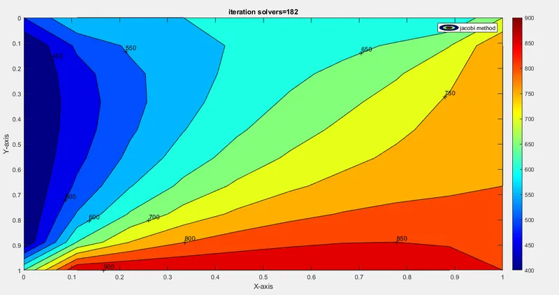
visuals :
gauss siedel method :
%solve steady state heat conduction equation in imlicit method
% by using iterative solvers -gauss seidel method
clear all
close all
clc

%length & the breadth of the given domain
l=1;
h=1;
%no of grid points that has been given
nx=10;
ny=nx;

x=linspace(0,l,nx);
y=linspace(0,h,ny);

dx=l/(nx-1);
dy=h/(ny-1);

%initila bounday conditions
T=600*ones(nx,ny);

%boundary conditions of the given domain
T_b=900;
T_t=600;
T_l=400;
T_r=800;

%defining all sides temperature values of the domain
T(1,1:end)=T_t;
T(end,1:end)=T_b;
T(1:end,1)=T_l;
T(:,end)=T_r;

%calculate the temperature values at  all the edges
T(1,end)=(T_r+T_t)/2;
T(1,1)=(T_t+T_l)/2;
T(end,1)=(T_b+T_l)/2;
T(end,end)=(T_r+T_b)/2;

% absolute error criteria is
tolerence=1e-4;
error=1;

Told=T;
k=((2*(dx^2+dy^2))/(dx^2*dy^2))*dx^2;

%calculating 2d heat conduction equation
%convergence loop
iteration_solver=2;
if iteration_solver==2
    gs_iter=1;
    while(error>tolerence)
        for i=2:nx-1
            for j=2:ny-1
                T(i,j)=0.25*(T(i+1,j)+T(i-1,j)+T(i,j+1)+T(i,j-1));
            end
        end
        error=max(max(abs(Told-T)));
        Told=T;
        gs_iter=gs_iter+1;

        figure(1)
        contourf(x,y,T)
        clabel(contourf(x,y,T))
        colorbar
        colormap(jet)
        set(gca,'ydir','reverse')
        xlabel('X-axis')
        ylabel('Y-axis')
        legend('gs method')
        title(sprintf('iteration solvers=%d',gs_iter));
        pause(0.003)
    end
end
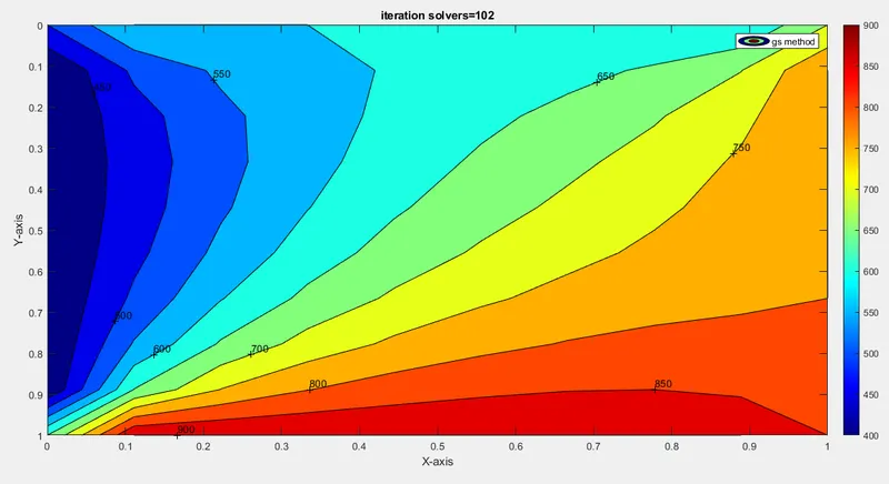
visuals :
successive over relaxation :
%solve steady state heat conduction equation in imlicit method
% by using iterative solvers -successive over relaxation method
clear all
close all
clc

%length & the breadth of the given domain
l=1;
h=1;
%no of grid points that has been given
nx=10;
ny=nx;

x=linspace(0,l,nx);
y=linspace(0,h,ny);

dx=l/(nx-1);
dy=h/(ny-1);

%initila bounday conditions
T=600*ones(nx,ny);

%boundary conditions of the given domain
T_b=900;
T_t=600;
T_l=400;
T_r=800;

%defining all sides temperature values of the domain
T(1,1:end)=T_t;
T(end,1:end)=T_b;
T(1:end,1)=T_l;
T(:,end)=T_r;

%calculate the temperature values at  all the edges
T(1,end)=(T_r+T_t)/2;
T(1,1)=(T_t+T_l)/2;
T(end,1)=(T_b+T_l)/2;
T(end,end)=(T_r+T_b)/2;

% absolute error criteria is
tolerence=1e-4;
error=1;

Told=T;
k=((2*(dx^2+dy^2))/(dx^2*dy^2))*dx^2;
omega=1.5;

%calculating 2d heat conduction equation
%convergence loop
iteration_solver=3;
if iteration_solver==3
    sor_iter=1;
    while(error>tolerence)
        for i=2:nx-1
            for j=2:ny-1
                T(i,j)=(1-omega)*Told(i,j)+omega*(0.25*(T(i+1,j)+T(i-1,j)+T(i,j+1)+T(i,j-1)));
            end
        end
        error=max(max(abs(Told-T)));
        Told=T;
        sor_iter=sor_iter+1;

        figure(1)
        contourf(x,y,T)
        clabel(contourf(x,y,T))
        colorbar
        colormap(jet)
        set(gca,'ydir','reverse')
        xlabel('X-axis')
        ylabel('Y-axis')
        legend('sor method')
        title(sprintf('iteration solvers=%d',sor_iter));
        pause(0.003)
    end
end
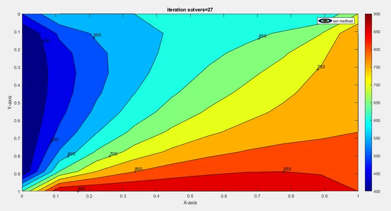
visuals:
unsteady state equation descritization :
temperature changes throughout the body with varying time so we will have to solve forward difference approximation for the time and the central difference approximation for the claculating the temperature at all the nodes.
`(T_(i,j)^(n+1)-T_(i,j)^n)/(Deltat)=alpha((T_(i+1,j)-2T_(i,j)+T_(i-1,j))/(Deltax^2)+(T_(i,j+1)-2T_(i,j)+T_(i,j-1))/(Deltay^2))`
i,j+1 is for top hand side approximation so that am taking that as an 't'
i,j-1 is for bottom hand side approximation so that am taking that as an 'b'
i,j is for current approximation so that am taking that as an 'p'
i+1,j is for right hand side approximation so that am taking that as an 'r'
i,j-1 is for left hand side approximation so that am taking that as an 'l'
i,j is for current approximation so that am taking that as an 'p'
so the above equation becomes;
`(T_p^(n+1)-T_p^n)/(Deltat)=alpha((T_r-2T_p+T_l)/(Deltax^2)+(T_t-2T_p+T_b)/(Deltay^2))`
`(T_p^(n+1)-T_p^n)=(alpha*(Deltat))/(Deltax^2)(T_r-2T_p+T_l)+(alpha*(Deltat))/(Deltay^2)(T_t-2T_p+T_b)`
`(alpha*(Deltat))/(Deltax^2)=k1`
`(alpha*(Deltat))/(Deltay^2)=k2`
`(T_p^(n+1)-T_p^n)=k1(T_r-2T_p+T_l)+k2(T_t-2T_p+T_b)`
if we write the above equation in implicit form the equation becomes
`(T_p^(n+1)-T_p^n)=k1(T_r-2T_p+T_l)^(n+1)+k2(T_t-2T_p+T_b)^(n+1)`
so we rewrite the eq in the below form
`T_p^n=T_p^(n+1)-k1*T_r^(n+1)+k1*2T_p^(n+1)-k1*T_l^(n+1)-k2*T_t^(n+1)+k2*2T_p^(n+1)-k2*T_b^(n+1)`
take common terms out,
`T_p^n=T_p^(n+1)(1+2*k1+2*k2)-k1*T_r^(n+1)-k1*T_l^(n+1)-k2*T_t^(n+1)-k2*T_b^(n+1)`
`T_p^(n+1)(1+2*k1+2*k2)=T_p^n+k1*T_r^(n+1)+k1*T_l^(n+1)+k2*T_t^(n+1)+k2*T_b^(n+1)`
`T_p^(n+1)=(1/(1+2*k1+2*k2))(T_p^n+k1*T_r^(n+1)+k1*T_l^(n+1)+k2*T_t^(n+1)+k2*T_b^(n+1))`
here `alpha`is a diffusivity term
If we write an equation in indices form ,
`T_(i,j)=(1/(1+2*k1+2*k2))(T_(i,j)+k1(T_(i+1,j)+T_(i-1,j))+k2(T_(i,j+1)+T_(i,j-1)))`
unsteady state jacobi method :
%solve unsteady state heat conduction equation in imlicit method
% by using iterative solvers -jacobi method
clear all
close all
clc
tic
%length & the breadth of the given domain
l=1;
h=1;
%no of grid points that has been given
nx=50;
ny=nx;
%n0 of time steps
nt=1400;
dt=1e-3;

x=linspace(0,l,nx);
y=linspace(0,h,ny);

dx=l/(nx-1);
dy=h/(ny-1);

%initila bounday conditions
T=600*ones(nx,ny);

%boundary conditions of the given domain
T_b=900;
T_t=600;
T_l=400;
T_r=800;

%defining all sides temperature values of the domain
T(1,1:end)=T_t;
T(end,1:end)=T_b;
T(1:end,1)=T_l;
T(:,end)=T_r;

%calculate the temperature values at  all the edges
T(1,end)=(T_r+T_t)/2;
T(1,1)=(T_t+T_l)/2;
T(end,1)=(T_b+T_l)/2;
T(end,end)=(T_r+T_b)/2;

% absolute error criteria is
tolerence=1e-4;
error=1;

Told=T;
Tprev=T;
omega=1.4;

k1=(omega*dt)/dx^2;
k2=(omega*dt)/dy^2;


%calculating 2d heat conduction equation for unsteady
%if statement
%time loop
%indicate to run till my solution converge(while)
%convergence loop
iteration_solver=1;
if iteration_solver==1
    jacobi_iter=1;
    for k=1:nt
        error=1;
        while(error>tolerence)
            for i=2:nx-1
                for j=2:ny-1
                    term1=1/(1+2*k1+2*k2);
                    term2=k1*term1;
                    term3=k2*term1;
                    H=((Told(i-1,j))+(Told(i+1,j)));
                    V=((Told(i,j-1))+(Told(i,j+1)));
                    T(i,j)=(Tprev(i,j)*term1)+term2*H+term3*V;
                end
            end
            error=max(max(abs(Told-T)));
            Told=T;
            jacobi_iter=jacobi_iter+1;
        end
        Tprev=T;
    end
end
figure(1)
contourf(x,y,T)
clabel(contourf(x,y,T))
colorbar
colormap(jet)
set(gca,'ydir','reverse')
xlabel('X-axis')
ylabel('Y-axis')
legend('jacobi method-unsteady')
title(sprintf('no of iterations=%d',jacobi_iter));
jacobi_time=toc;
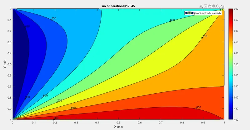
plot :
gauss-siedel method :
%solve unsteady state heat conduction equation in imlicit method
% by using iterative solvers -gauss seidel method
clear all
close all
clc
tic
%length & the breadth of the given domain
l=1;
h=1;
%no of grid points that has been given
nx=50;
ny=nx;
%n0 of time steps
nt=1400;
dt=1e-3;

x=linspace(0,l,nx);
y=linspace(0,h,ny);

dx=l/(nx-1);
dy=h/(ny-1);

%initila bounday conditions
T=600*ones(nx,ny);

%boundary conditions of the given domain
T_b=900;
T_t=600;
T_l=400;
T_r=800;

%defining all sides temperature values of the domain
T(1,1:end)=T_t;
T(end,1:end)=T_b;
T(1:end,1)=T_l;
T(:,end)=T_r;

%calculate the temperature values at  all the edges
T(1,end)=(T_r+T_t)/2;
T(1,1)=(T_t+T_l)/2;
T(end,1)=(T_b+T_l)/2;
T(end,end)=(T_r+T_b)/2;

% absolute error criteria is
tolerence=1e-4;
error=1;

Told=T;
Tprev=T;
omega=1.4;

k1=(omega*dt)/dx^2;
k2=(omega*dt)/dy^2;


%calculating 2d heat conduction equation for unsteady
%if statement
%time loop
%indicate to run till my solution converge(while)
%convergence loop
iteration_solver=1;
if iteration_solver==1
    gs_iter=1;
    for k=1:nt
        error=1;
        while(error>tolerence)
            for i=2:nx-1
                for j=2:ny-1
                    term1=1/(1+2*k1+2*k2);
                    term2=k1*term1;
                    term3=k2*term1;
                    H=((T(i-1,j))+(T(i+1,j)));
                    V=((T(i,j-1))+(T(i,j+1)));
                    T(i,j)=(Tprev(i,j)*term1)+term2*H+term3*V;
                end
            end
            error=max(max(abs(Told-T)));
            Told=T;
            gs_iter=gs_iter+1;
        end
        Tprev=T;
    end
end
figure(1)
contourf(x,y,T)
clabel(contourf(x,y,T))
colorbar
colormap(jet)
set(gca,'ydir','reverse')
xlabel('X-axis')
ylabel('Y-axis')
legend('gs method-unsteady')
title(sprintf('no of iterations=%d',gs_iter));
gs_time=toc;
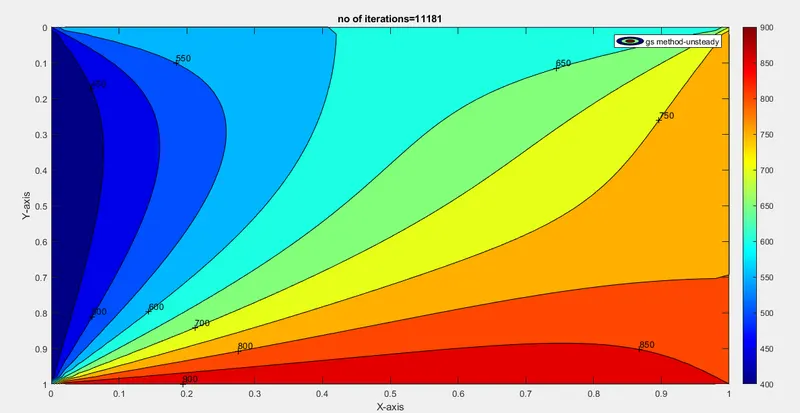
plot:
successive over rrelaxaion method :
%solve unsteady state heat conduction equation in imlicit method
% by using iterative solvers -successive over relaxation method
clear all
close all
clc
tic
%length & the breadth of the given domain
l=1;
h=1;
%no of grid points that has been given
nx=50;
ny=nx;
%no of time steps
nt=1400;
dt=1e-3;

x=linspace(0,l,nx);
y=linspace(0,h,ny);

dx=l/(nx-1);
dy=h/(ny-1);

%initila bounday conditions
T=600*ones(nx,ny);

%boundary conditions of the given domain
T_b=900;
T_t=600;
T_l=400;
T_r=800;

%defining all sides temperature values of the domain
T(1,1:end)=T_t;
T(end,1:end)=T_b;
T(1:end,1)=T_l;
T(:,end)=T_r;

%calculate the temperature values at  all the edges
T(1,end)=(T_r+T_t)/2;
T(1,1)=(T_t+T_l)/2;
T(end,1)=(T_b+T_l)/2;
T(end,end)=(T_r+T_b)/2;

% absolute error criteria is
tolerence=1e-4;
error=1;
Told=T;
Tprev=T;
omega=1.4;

k1=(omega*dt)/dx^2;
k2=(omega*dt)/dy^2;


%calculating 2d heat conduction equation for unsteady
%if statement
%time loop
%indicate to run till my solution converge(while)
%convergence loop
iteration_solver=1;
if iteration_solver==1
    sor_iter=1;
    for k=1:nt
        error=1;
        term1=(1/(1+2*k1+2*k2));
        term2=k1*term1;
        term3=k2*term1;
        while(error>tolerence)
            for i=2:nx-1
                for j=2:ny-1

                    H=(T(i-1,j))+(Told(i+1,j));
                    V=(T(i,j-1))+(Told(i,j+1));
                    T(i,j)=(1-omega)*Told(i,j)+omega*((Tprev(i,j)*term1)+(term2*H)+(term3*V));

                end
            end
            error=max(max(abs(Told-T)));
            Told=T;
            sor_iter=sor_iter+1;
        end
        Tprev=T;
    end
end
figure(1)
contourf(x,y,T)
clabel(contourf(x,y,T))
colorbar
colormap(jet)
set(gca,'ydir','reverse')
xlabel('X-axis')
ylabel('Y-axis')
legend('sor method-unsteady')
title(sprintf('no of iterations=%d',sor_iter));
sor_time=toc;
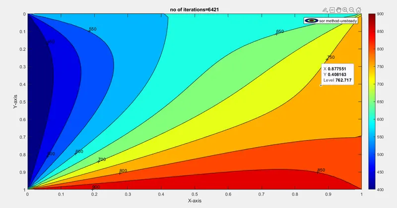
plot :
explicit form of the unsteady state of 2d heat conduction rquation :
`(T_p^(n+1)-T_p^n)=k1(T_r-2T_p+T_l)+k2(T_t-2T_p+T_b)`
`(T_p^(n+1)-T_p^n)=k1(T_r-2T_p+T_l)^n+k2(T_t-2T_p+T_b)^n`
program:
%solve unsteady state heat conduction equation in explicit method
clear all
close all
clc
tic
%length & the breadth of the given domain
l=1;
h=1;
%no of grid points that has been given
nx=10;
ny=nx;
%n0 of time steps
nt=1400;
dt=1e-3;

x=linspace(0,l,nx);
y=linspace(0,h,ny);

dx=l/(nx-1);
dy=h/(ny-1);

%initila bounday conditions
T=600*ones(nx,ny);

%boundary conditions of the given domain
T_b=900;
T_t=600;
T_l=400;
T_r=800;

%defining all sides temperature values of the domain
T(1,1:end)=T_t;
T(end,1:end)=T_b;
T(1:end,1)=T_l;
T(:,end)=T_r;

%calculate the temperature values at  all the edges
T(1,end)=(T_r+T_t)/2;
T(1,1)=(T_t+T_l)/2;
T(end,1)=(T_b+T_l)/2;
T(end,end)=(T_r+T_b)/2;

% absolute error criteria is
tolerence=1e-4;
error=1;

Told=T;
omega=1.4;

k1=(omega*dt)/dx^2;
k2=(omega*dt)/dy^2;


%calculating 2d heat conduction equation for unsteady
%if statement
%time loop
%indicate to run till my solution converge(while)
%convergence loop
iteration_solver=1;
if iteration_solver==1
    explicit_iterations=1;
    for k=1:nt
        error=1;
        while(error>tolerence)
            for i=2:nx-1
                for j=2:ny-1
                   T(i,j)=Told(i,j)+k1*(Told(i-1,j)-2*Told(i,j)+Told(i+1,j))+k2*(Told(i,j-1)-2*Told(i,j)+Told(i,j+1));
                end
            end
            error=max(max(abs(Told-T)));
            Told=T;
            explicit_iterations=explicit_iterations+1;
        end
    end
end
figure(1)
contourf(x,y,T)
clabel(contourf(x,y,T))
colorbar
colormap(jet)
set(gca,'ydir','reverse')
xlabel('X-axis')
ylabel('Y-axis')
legend('explicit method-unsteady')
title(sprintf('no of iterations=%d',explicit_iterations));
explicit_iterations=toc;
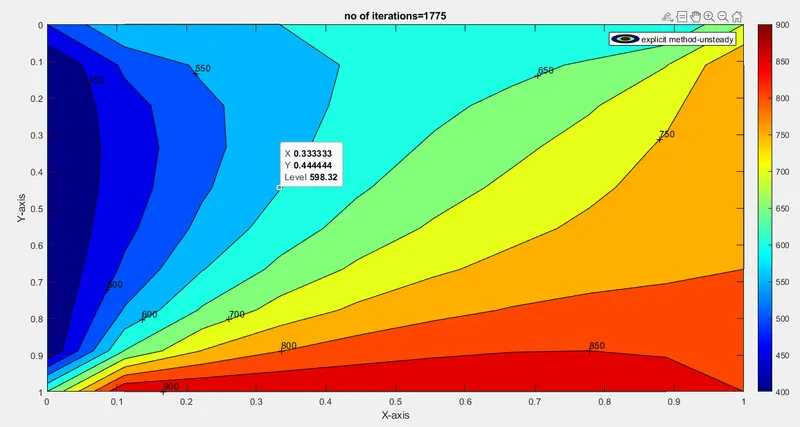
plot :
program explanation :
1)initially i have defined all the nodes on both the axis since it is 2 dimensional.and also defined temperature values at all the nodes.and after i have defined all the corner node temperature by taking average of the respective boundary temperatures.and also the length and breadth dimensions of the 2d plate.then i have tried to find out the dx and dy values.and also defined the boundary conditions.
2)we have used iteration solvers to identify the best possible solutions.so i have used if condition to define the method of the solver and also define the tolerance values as 1e-4 and the error as 1 by using while loop we were able to run the simulation till the error value is greater than tolerance.define node conditions by using for loops for both and define the formula inside the loop and end the nodes loops and define old temperature values as new temperature values.so that we will get the converge solution accordingly.and also define error value
3)for unsteady 2d heat conduction equation we have added time steps to converge the solution.
4)after plotting i have included the no of iterations also inside the plot so that we can clearly absorve that the no of iterations taken by the solver and also compare that the iteration solver method definition applies or not.
conclusion :
i have taken 50 grid points for unsteady state so that only i am able satisfy the logic of iterstion solvers .while taking 1o nodes.i was not able satisfy the condition for successie over relaxation method,the condition must be iteratons of jacobi solver >iterations of gauss seidel > iterations of successive over relaxation.s, that i took 50nodes and solve the equation.
steady state 2d heat conduction equation for 10 nodes :(implicit method)
no of iterations for jacobi method -182
no of iterations for gauss seidel method -102
no of iterations for successive over relaxation method -27
unsteady state 2d heat conduction equation for 10 nodes :(implicit method)
no of iterations for jacobi method -6421
no of iterations for gauss seidel method -11181
no of iterations for successive over relaxation method -17645
unsteady state 2d heat conduction equation for 10 nodes :(explicit method)
we need not to use any iteration solver here,because we are solving the present temperature value by using the previous time time step value.
no of iterations =1775