Week 5.1 - Mid term project - Solving the steady and unsteady 2D heat conduction problem
Aim: To create 2D steady and transient heat conduction equation solver in MATLAB with the help of iterative solvers.
Objective :
1) Discreatize 2d heat conduction equation into system of linear algebraic equations
2) apply iterative solvers to this equations
3) create MATLAB code for solving this equations
4) Plotting and analysing solutions by different methods.
(1) 2D -Steady State Heat Conduction Equation
`(del^2T)/(delx^2) + (del^2T)/(dely^2) = 0`
discreatizing this equation we get ,
`T(i,j) = 1/k *(T(i-1,j) + T(i+1,j))/(deltax^2) +1/k *(T(i,j-1) + T(i,j+1))/(deltay^2)`
Solving This equation by iterative techniques
1)Jacobi
2) gauss seidel
3) Succesive over relaxation
Main Programme :
close all
clear all
clc

%% Solving 2D Heat Conduction Equation (steady state)

% equation is (d^2T/dx^2 + d^T/dy^2) = 0
%% inputs
L = 1;
nx = 100; % nodes in x axis
ny = 100; % nodes in y axis
x = linspace(0,L,nx);
y = linspace(0,L,ny);
dx = x(2) -x(1);
dy = y(2)-y(1);
%% Defining Boundary Conditions
TBC = 600 ; % Top BCs
BBC =900;  % Bottom BCs
LBC = 400; % Left BCs
RBC = 800; % Right BCs
%% Creating temperature Domain
T = 300*ones(nx,ny);
T(1,:)= TBC;
T(end,:) = BBC;
T(:,1) = LBC;
T(:,end) = RBC;

Told = T ;
Tin = T;
%% Specifying iterative method
iteration_method =1
error = 9;
tol = 1e-4;
%% Jacobi Method

%Convergence loop
if iteration_method==1 % Jacobi Method
    iter =1
    tic
while (error> tol)
     for i = 2:nx-1
      for  j = 2:ny-1

        k = (2.*(dx.^2 +dy.^2))./((dx.^2).*(dy.^2));
        term1(i,j) = (T(i-1,j) + T(i+1,j))./(dx.^2);
        term2(i,j) = (T(i,j-1) + T(i,j+1))./(dy.^2);
        T(i,j) = (1./k).*(term1(i,j)) + (1./k).*(term2(i,j));
      end
     end

     error = max(max(abs(Told-T)));
     Told = T;
   iter = iter +1


end
time =toc ;

%% Gauss Seidal Method
elseif iteration_method==2 % gauss seidel method;
    iter =1;
    tic
    while (error> tol)
     for i = 2:nx-1
      for  j = 2:ny-1

        k = (2.*(dx.^2 +dy.^2))./((dx.^2).*(dy.^2));
        term1(i,j) = (T(i-1,j) + Told(i+1,j))./(dx.^2);
        term2(i,j) = (T(i,j-1) + Told(i,j+1))./(dy.^2);
        T(i,j) = (1./k).*(term1(i,j)) + (1./k).*(term2(i,j));
      end
     end

     error = max(max(abs(Told-T)));
     Told = T;
   iter = iter +1
    end
time =toc ;

%% Succesive Over Relaxation Method
elseif iteration_method ==3 % Succesive over relaxation
    iter =1;
    tic
    omega =1.8;
      while (error> tol)
     for i = 2:nx-1
      for  j = 2:ny-1
     k = (2.*(dx.^2 +dy.^2))./((dx.^2).*(dy.^2));
        term1(i,j) = (T(i-1,j) + Told(i+1,j))./(dx.^2);
        term2(i,j) = (T(i,j-1) + Told(i,j+1))./(dy.^2);
        T(i,j) = (1./k).*(term1(i,j)) + (1./k).*(term2(i,j));
        T(i,j) = (1-omega)*Told(i,j) + omega*(T(i,j));
      end
     end

     error = max(max(abs(Told-T)));
     Told = T;
     iter= iter +1;
      end
end
time = toc

%% Plotting
[c,h] = contourf(x,y,T)
clabel(c,h)
colorbar

title({['iteration Method =',num2str(iteration_method)];['Number of iterations =',num2str(iter)];['Simulation run time =',num2str(time)]});
ax =gca ;
ax.YDir = 'reverse';
xlabel('X-axis') ;
ylabel('Y-axis');
Explanation Of Code :
1) input conditions are specified and domain is created
2) Temperature domain is created using ones command and guess of 300 is selected.
3) Boundary Conditions of temperature are given
4) error and tolerance values are specified
5) if iteration method =1 then jacobi method is used ,if iteration method =2 then gauss seidel method is used , if iteration method =3 then SOR is used
6) convergence loop is created using while and space loop is created using for
7) error is calculated after each space loop untill error is less than tolerance value which is 1e-4
8) Plotting is done using contourf command
Results :
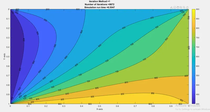
1) Jacobi Method
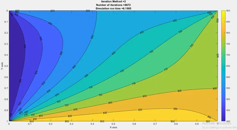
2) Gauss Seidel Method
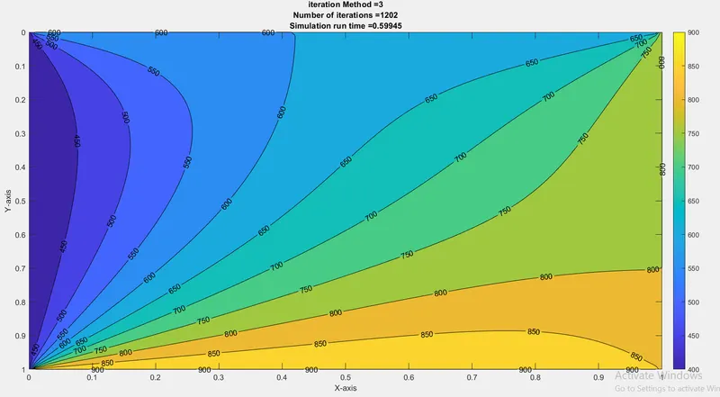
3) Succesive Over Relaxation Method :
Explanation :
from plots we can observe that SOR method is faster than other two methods hence solution converges really fast if we use this method. gauss seidel method is faster than jacobi method
2) Transient 2D Heat Conduction :
`(delT)/(delt) = (del^2T)/(delx^2) + (del^2T)/(dely^2)`
By discreatizing this equation we get
`(Tp^(n+1) - Tp)/(deltat) = alpha * (( TL -2Tp +TR)/(deltax^2) + ( Tt -2Tp +Tb)/(deltay^2)) ^(n+1)`
Solving by IMPLICIT Method
Main Programme :
close all
clear all
clc
%% Inputs
L = 1 ; % Length of domain
nx = 100;
ny =100 ;
t =1000 ; % time
nt = 1400; % no. of time steps
x = linspace(0,L,nx) ;
y = linspace(0,L,ny);
dx =  x(2)-x(1) ;
dy = y(2) - y(1) ;
dt = t/nt;

%% Temperature grid/domain  generation
T = 300*ones(nx,ny);
%% Boundary Conditions
TBC = 600 ;
BBC =900;
LBC = 400;
RBC = 800;
T(1,:)= TBC;
T(end,:) = BBC;
T(:,1) = LBC;
T(:,end) = RBC;
Told = T;
Tprev = T;
a = 1.75e-4;
k1 = (a*dt)./(dx^2);
k2 = (a*dt)./(dy^2);
CFL = a.*dt.*((1./dx^2) + (1/dy^2));


tol = 1e-4;
iter = 1 ;
%% specifying iteration method
iteration_method = 3;
%% Jacobi Method
if iteration_method ==1
    tic
    % time loop
for n = 1:nt
    %%Convergence loop
  error = 1;
    while (error>tol)
        %Space loop
        for i =2:nx-1 ;
            for j = 2: ny-1
                term1 = 1./(1+2*k1 +2*k2);
                H = Told(i-1,j) + Told(i+1,j);
                V = Told(i,j-1) + Told(i,j+1);
                term2 = k1*term1 ;
                term3 = k2*term1;
                T(i,j) = Tprev(i,j)*term1 + term2*H + term3*V ;
            end
        end
        error = max(max(abs(Told - T)));
        Told = T ;
     iter = iter +1
    end
    Tprev = T ;
end

  time = toc ;


  %% Gauss seidel  Method
elseif iteration_method ==2
    tic
    % time loop
for n = 1:nt
    %%Convergence loop
  error = 1;
    while (error>tol)
        %Space loop
        for i =2:nx-1 ;
            for j = 2: ny-1
                term1 = 1./(1+2*k1 +2*k2);
                H = T(i-1,j) + Told(i+1,j);
                V = T(i,j-1) + Told(i,j+1);
                term2 = k1*term1 ;
                term3 = k2*term1;
                T(i,j) = Tprev(i,j)*term1 + term2*H + term3*V ;
            end
        end
        error = max(max(abs(Told - T)));
        Told = T ;
     iter = iter +1
    end
    Tprev = T ;
end


  time = toc ;


    %% Succesive Over Relaxat;ion Method
elseif iteration_method ==3
    tic
    omega = 1.5;
    % time loop
for n = 1:nt
    %%Convergence loop
  error = 1;
    while (error>tol)
        %Space loop
        for i =2:nx-1 ;
            for j = 2: ny-1
                term1 = 1./(1+2*k1 +2*k2);
                H = T(i-1,j) + Told(i+1,j);
                V = T(i,j-1) + Told(i,j+1);
                term2 = k1*term1 ;
                term3 = k2*term1;
                T(i,j) = Tprev(i,j)*term1 + term2*H + term3*V ;
                T(i,j) = (1-omega)*Told(i,j) + omega*(T(i,j));
            end
        end
        error = max(max(abs(Told - T)));
        Told = T ;
     iter = iter +1
    end
    Tprev = T ;
end
time = toc;
end
  %% plotting
[c,h] = contourf(x,y,T)
clabel(c,h)
colorbar

title({['iteration Method =',num2str(iteration_method)];['Number of iterations =',num2str(iter)];['Simulation run time =',num2str(time)]});
ax =gca ;
ax.YDir = 'reverse';
xlabel('X-axis') ;
ylabel('Y-axis');
Explanation of Code :
1) input conditions are specified and domain is created
2) Temperature domain is created using ones command and guess of 300 is selected.
3) Boundary Conditions of temperature are given
4) error and tolerance values are specified
5) if iteration method =1 then jacobi method is used ,if iteration method =2 then gauss seidel method is used , if iteration method =3 then SOR is used
6) convergence loop is created using while and space loop is created using for
7) Time loop is created for getting time marching solution
8) error is calculated after each space loop untill error is less than tolerance value which is 1e-4
9) Plotting is done using contourf command
Results :
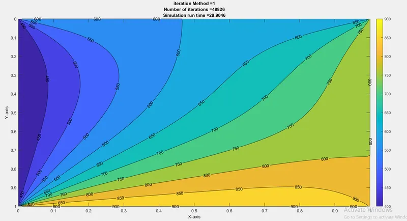
1) Jacobi Method
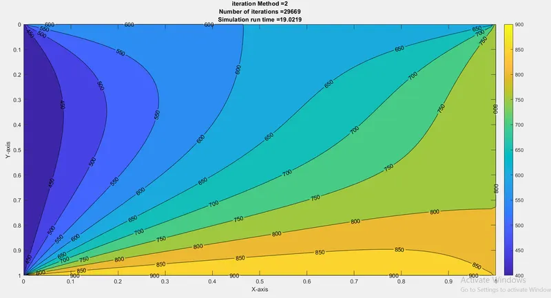
2) Gauss seidel Method :
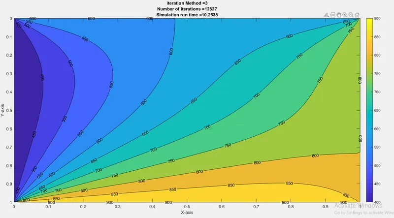
3) Succesive over relaxation method
Explanation :
from plots we can observe that SOR method is faster than other two methods hence solution converges really fast if we use this method. gauss seidel method is faster than jacobi method