Week 5.1 - Mid term project - Solving the steady and unsteady 2D heat conduction problem
Objective :
1)
a) To solve 2D steady state equation using steady state analysis using point iterative technique (1.Jacobi 2. Gauss seidel 3. Successive over relaxation)
b) To solve 2D steady state equation using transient state analysis using explicit and implicit method .
2) To plot graph for temperature variation within the grid plane for all the cases .
Theory :
Explicit method :
In an explicit approach , each difference equation contains only 1 unknown and be therefore solved explicitly for this unknown in a straight forward manner .
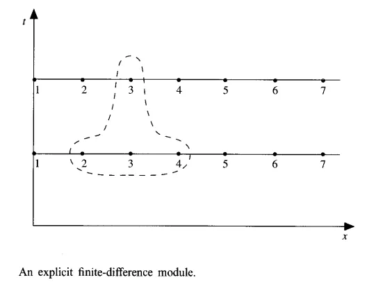
Equation for explicit with unkown on LHS and known on RHS

Implicit Method :
Implicit approach is one where the unknowns must br obtained by means of a simultaneous solution of the difference equation applied at all grid points arrayed at a given time level .
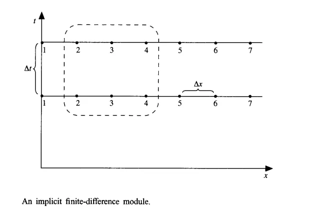
Equation for implicit method with unknowns on LHS and knowns on RHS
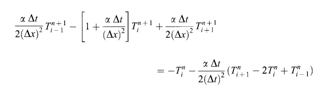
We can iteratively obtain solution using implicit scheme using 3 methods
a) Jacobi Method :
Equation for Jacobi method is as follows
`T(i,j)= 1/k (T_(old)(i-1,j)+T_(old)(i+1,j))/(trianglex^2) + 1/k (T_(old)(i,j-1)+T_(old)(i,j+1))/(triangley^2)`
b)Gauss Seidel method
Equation for Gauss Seidel method is as follows
`T(i,j)= 1/k (T(i-1,j)+T_(old)(i+1,j))/(trianglex^2) + 1/k (T(i,j-1)+T_(old)(i,j+1))/(triangley^2)`
c)Successive over relaxation
Equation for SOR is as follows .
`T(i,j) = (1-omega)*T_(old) + omega*T_(GS)`
Governing Equation :
2D steady state heat conduction equation
`(del^2 T) / (delx^2) + (del^2 T)/(dely^2) = 0`
Since it is a steady state equation , time term is 0 and diffusivity is constant .
From equation , we can observe that it is elliptic since `b^2-4ac <0`
2D transient state heat conduction equation
`(delT)/(delt) + alpha *((del^2T)/(delx^2)+(del^2T)/(dely^2))=0`
Here the equation is hyperbolic as time/information is travelling only in 1 direction .
Boundary Condition :
Here the boundary condition is given as
T_left = 400K
T_right=800K
T_top=600K
T_bottom=900K
Initial condition is entered as 300K .
Discretization scheme :
i) Steady state condition
Using iterative solver , the equation is as follows
a) Jacobi Method :
Equation for Jacobi method is as follows
`T(i,j)= 1/k (T_(old)(i-1,j)+T_(old)(i+1,j))/(trianglex^2) + 1/k (T_(old)(i,j-1)+T_(old)(i,j+1))/(triangley^2)`
b)Gauss Seidel method
Equation for Gauss Seidel method is as follows
`T(i,j)= 1/k (T(i-1,j)+T_(old)(i+1,j))/(trianglex^2) + 1/k (T(i,j-1)+T_(old)(i,j+1))/(triangley^2)`
c)Successive over relaxation
Equation for SOR is as follows .
`T(i,j) = (1-omega)*T_(old) + omega*T_(GS)`
ii) Transient state condition
Here we use forward differencing scheme as time or info travels only in one direction (forward)
for explicit method
`T_(i,j)^(n+1)= T_(i,j)^n+k1*(T_(i-1,j)-2T_(i,j)+T_(i+1,j))^n+k2(T_(i,j+1)-2T_(i,j)+T_(i,j-1))^n`
where
`k1=(alpha*trianglet)/(trianglex^2)`
`k2= (alpha*trianglet)/(triangley^2)`
For implicit method
`T_(i,j)^(n+1)= T_(i,j)^n+k1*(T_(i-1,j)-2T_(i,j)+T_(i+1,j))^(n+1)+k2(T_(i,j+1)-2T_(i,j)+T_(i,j-1))^(n+1)`
Program Code :
a) Steady state
clear all
close all
clc

nx=10;
ny=10;
t=ones(nx,ny);


t(1,1:ny)=600;
method=0;
t(1:nx,1)=400;
t(1:nx,ny)=800;
t(nx,1:ny)=900;
t(1,1)=500;
t(10,1)=650;
t(1,10)=700;
t(10,10)=850;
t(2:nx-1,2:ny-1)=300;
x=linspace(0,1,nx);
y=linspace(0,1,ny);
dx= 1/(nx-1);
dy=1/(ny-1);
[xx yy]=meshgrid(x,y);
k=(2*(dx^2+dy^2)/((dx^2)*(dy^2)));
error=9e9;
tol=1e-4;
told1=t;
told2=t;
told3=t;
% t2=t;
tinitial=t;
j_iter=1;
gs_iter=1;
sor_iter=1;
w=0;
method=input('Enter method number 1.Jacobi 2.Gauss Seidel 3.SOR')
%Jacobi
if (method==1)
while error>tol

for i=2:nx-1
    for j=2:ny-1
        term1= (told1(i-1,j)+told1(i+1,j))/(dx^2);
        term2= (told1(i,j-1)+told1(i,j+1))/(dy^2);
        t(i,j)=(term1+term2)/k ;
    end
end
a = ((t-told1))
b=max(max(a))

error=b
told1=t;
j_iter=j_iter+1;
end

contourf(x,y,t,'showtext','on')
colormap(jet)
colorbar
set(gca,'YDIR','reverse')

xlabel('X axis')
ylabel('Y axis')
title(sprintf('2D steady state analysis (Jacobi) for %d number of iterations ',j_iter))
pause(0.02)

end
%Gauss Seidel
if(method==2)
    while error>tol

for i=2:nx-1
    for j=2:ny-1
        term1= (t(i-1,j)+told2(i+1,j))/(dx^2);
        term2= (t(i,j-1)+told2(i,j+1))/(dy^2);
        t(i,j)=(term1+term2)/k ;
    end
end
a = ((t-told2))
b=max(max(a))
error=b
told2=t;
gs_iter=gs_iter+1;
end
contourf(x,y,t,'showtext','on')
colormap(jet)
colorbar
set(gca,'YDIR','reverse')

xlabel('X axis')
ylabel('Y axis')
title(sprintf('2D steady state analysis (Gauss Seidel) for %d number of iterations ',gs_iter))
pause(0.02)
end

% Successive Over-relaxation
if(method==3)
    w=input('Enter omega value >1 for succesive over relaxation')
    while error>tol

for i=2:nx-1
    for j=2:ny-1
        term1= (t(i-1,j)+told3(i+1,j))/(dx^2);
        term2= (t(i,j-1)+told3(i,j+1))/(dy^2);
         t(i,j)=(term1+term2)/k ;
        t(i,j)=(1-w)*told3(i,j) + w.*t(i,j) ;
    end
end
a = abs((t-told3))
b=max(max(a))
error=b
told3=t;
sor_iter=sor_iter+1;
end
contourf(x,y,t,'showtext','on')
colormap(jet)
colorbar
set(gca,'YDIR','reverse')

xlabel('X axis')
ylabel('Y axis')
title(sprintf('2D steady state analysis (SOR) for %d number of iterations ',sor_iter))
pause(0.02)
end
b) Transient Condition
clear all
close all
clc
% To create a 10x10 matrix or domain of study with given boundary condition
nx=10;
ny=10;
t=ones(nx,ny);


t(1,1:ny)=600;
method=0;
t(1:nx,1)=400;
t(1:nx,ny)=800;
t(nx,1:ny)=900;
t(1,1)=500;
t(10,1)=650;
t(1,10)=700;
t(10,10)=850;
t(2:nx-1,2:ny-1)=300;
x=linspace(0,1,nx);
y=linspace(0,1,ny);
dx= 1/(nx-1);
dy=1/(ny-1);
[xx yy]=meshgrid(x,y);
% k=(2*(dx^2+dy^2)/((dx^2)*(dy^2)));
error=9e9;
tol=1e-4;
told=t;
told2=t;
tp=t;
told3=t;
% t2=t;
tinitial=t;
j_iter=1;
gs_iter=1;
sor_iter=1;
w=0;
a1=1.5;
t_tot=10;
dt=2
nt=t_tot/dt;
%nt=30;
k=a1*dt/(dx^2);
%CFL number to check for stability condition
CFL=a1*dt/(dx^2);

method=input('enter method 1.explicit 2.implicit jacobi 3.implicit Gauss seidel 4. implicit SOR');

if(method==1)
    a1=0.02;
t_tot=10;
dt=0.1;
nt=t_tot/dt;
%nt=30;
k=a1*dt/(dx^2);
CFL=a1*dt/(dx^2);
% Explicit scheme

for o=1:nt

    for i=2:nx-1

        for j=2:ny-1

        term1= (told(i-1,j)-(2*told(i,j))+told(i+1,j));
        term2= (told(i,j-1)-(2*told(i,j))+told(i,j+1));
         t(i,j)=told(i,j)+k*(term1+term2) ;

        end
    end


error =max(max(abs(told-t)));
told=t;
end
% To plot contour (same code for all cases)
contourf(x,y,t,'showtext','on')

colormap(jet)
colorbar
set(gca,'YDIR','reverse')
xlabel('X axis')
ylabel('Y axis')
title(sprintf('2D transient analysis by explicit method'))
pause(0.02)
end
%Implicit scheme
if (method==2)


    % Time step iteration (for all cases)
     for o=1:nt
   while error>tol
    % Space step iteration (for all cases )
for i=2:nx-1
    for j=2:ny-1
        term1=(1+(4*k))^-1;
        term2=k*term1;
        H=(told(i-1,j)+told(i+1,j));
        V=(told(i,j-1)+told(i,j+1));
        t(i,j)=(tp(i,j)*term1)+(H*term2)+(V*term2);
    end
end
a = abs((t-told))
b=max(max(a))
error=b
told=t;
j_iter=j_iter+1;
end
tp=told;
     end

   contourf(x,y,t,'showtext','on')

colormap(jet)
colorbar
set(gca,'YDIR','reverse')
xlabel('X axis')
ylabel('Y axis')
title(sprintf('2D transient analysis by implicit Jacobi method'))
pause(0.02)
end
% Gauss Seidel

if (method==3)

     for o=1:nt
   while error>tol

for i=2:nx-1
    for j=2:ny-1
        term1=(1+(4*k))^-1;
        term2=k*term1;
        H=(t(i-1,j)+told2(i+1,j));
        V=(t(i,j-1)+told2(i,j+1));
        t(i,j)=(tp(i,j)*term1)+(H*term2)+(V*term2);

    end
end
a = abs((t-told2))
b=max(max(a))
error=b
told2=t;
gs_iter=gs_iter+1;
end
tp=told;
     end

   contourf(x,y,t,'showtext','on')

colormap(jet)
colorbar
set(gca,'YDIR','reverse')
xlabel('X axis')
ylabel('Y axis')
title(sprintf('2D transient analysis by implicit Gauss Seidel method'))
pause(0.02)
end
%SOR

if (method==4)
    w=input('Enter omega value  for succesive over relaxation')
     for o=1:nt
   while error>tol

for i=2:nx-1
    for j=2:ny-1
        term1=(1+(4*k))^-1;
        term2=k*term1;
        H=(t(i-1,j)+told3(i+1,j));
        V=(t(i,j-1)+told3(i,j+1));
        t(i,j)=(tp(i,j)*term1)+(H*term2)+(V*term2);
         t(i,j)=(1-w)*told3(i,j) + w.*t(i,j)
    end
end
a = abs((t-told3))
b=max(max(a))
error=b
told3=t;
sor_iter=sor_iter+1;
end
tp=told;
     end

   contourf(x,y,t,'showtext','on')


colormap(jet)
colorbar
set(gca,'YDIR','reverse')
xlabel('X axis')
ylabel('Y axis')
title(sprintf('2D transient analysis by implicit SOR method'))
pause(0.02)
end
Output :
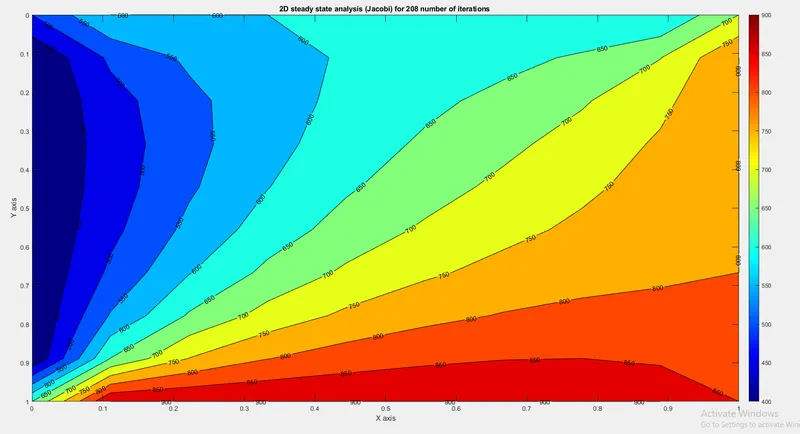
Program was written and contours were plotted for all cases .
1) Steady state
i) Jacobi
ii) Gauss seidel
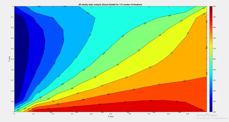
iii) Successive over-relaxation
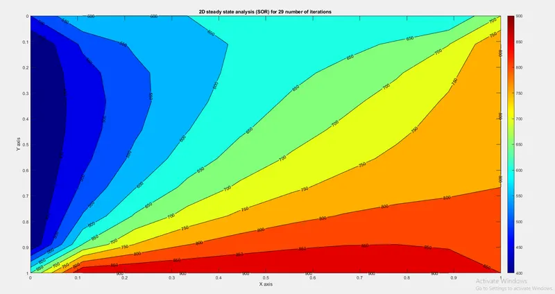
2) Transient Condition
a) Explicit scheme
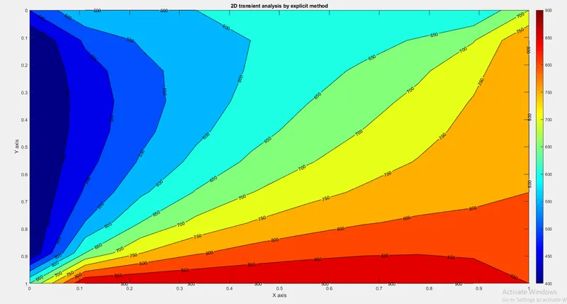
b) Implicit scheme
i) Jacobi
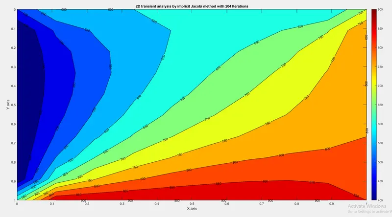
ii) Gauss Seidel
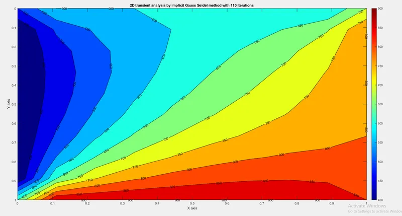
iii) Successive Over relaxation with `omega =1.5`
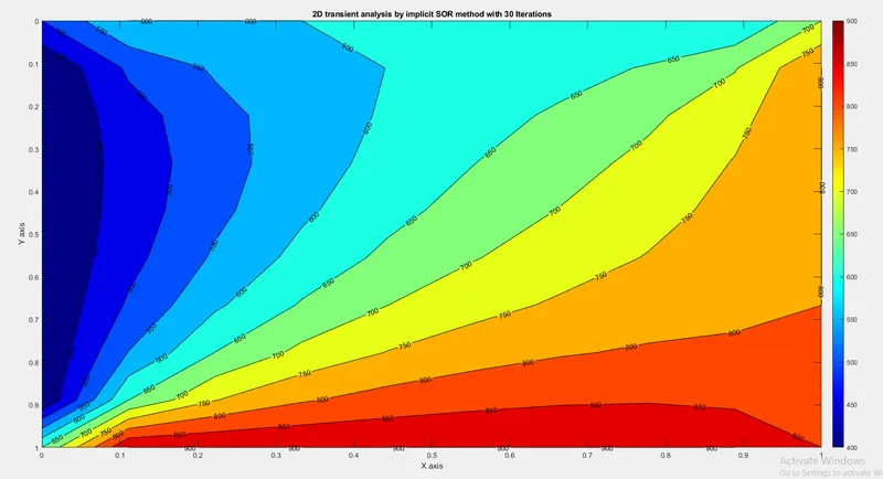
Inference :
From plotting all the contours , we have derived the same solution using different schemes and techniques .
Iterations for Jacobi>Gauss Seidel>Successive over-relaxation .