Week 5.1 - Mid term project - Solving the steady and unsteady 2D heat conduction problem

AIM: To obtain temperature distribution for a thin square plate by solving 2D heat conduction equation.

Objectives:

• To solve for 2D heat conduction equation for steady and unsteady state by explicit and implicit method with given boundary conditions.
• By implicit method- solve using different solvers i.e Jacobi, Gauss-Siedel, and Successive over relaxation(SOR) for both steady and transient state heat conduction equation.
• The accuracy of the solution obtained in both explicit and implicit method should be in accordance with the tolerance value mentioned.

Boundary Conditions:

Bottom Boundary=900k

Right boundary=800k

Left boundary=400k

Tolerance Value=1e-4.

Theory:

Numerical solution schemes are often reffered to as being explicit or implicit. When a direct computation of the dependent variables can be made in terms of known quantities, the computation is said to be explicit. When the dependent variables are defined by coupled sets of equations, and either a matrix or iterative technique is needed to obtain the solution, the numerical method is said to be implicit.

Explicit Method:

When a direct computation is made for an unknown quantity in terms of known quantity. This computation is called Explicit. This method requires stability criteria which when satisfied leads to stable solution. Because of the stabality criteria small time steps has to be taken to obtain stable solutions. With decrease in time step, the number of computations increases and hence computational time required for the solution to converge is less and the accuracy of the solution is high.

Implicit Method:

When a computation is made for dependent variable are defined by set of equations and a matrix is involved to find the unknown variable. This computation is called implicit method. This method is unconditionally stable as a result, no stability criteria is required to obtain a stable results and the computational time required for the solution to converge is high and accuracy of the solution is less relative to explicit method because this method uses simultaneous equations and uses guess values as the initial values to find the approximate values. If the guesses values are closer to the desired value the computational time is less. As there is no stability criteria requirement larger time steps can be used.

In order to solve for dependent variables iterative solvers used are

1. Jacobi Iterative solver

2.Gauss seidel iterative solver

3.Successive over relaxation iterative solver.

1. Jacobi Iterative solver-

In this method the temperature at (n+1)th term iteration is found using old values of the temperature defined at n'th term iteration. Using the approximation obtained iterations procedure it continued until desired accuracy of the solution is obtained.

2.Gauss seidel iterative solver

In this type iterative solver, temperature at n+1th iterations uses values of n+1 iterations that have already been computed. By this way old approximated values are overwritten with new approximate values for the iterations performed. Unlike jacobi, Gauss seidel require one storage vector which can be overwritten with each computation. This helps for the solution to converge faster than jacobi method.

3.Successive over relaxation iterative solver.

In this type of iterative solver relaxation factor is used in increasing the convergence rate. It goes by the formula

where `omega overset('')() >( (partialt)/(partialx^2) + (partialt)/(partialy^2))` is the relaxation factor.

Solving 2D heat conduction equation for steady state:

Governing eqution for 2D heat conduction equation for steady state is

`(partial^2T)/(partialx^2)+(partial^2T)/(partialy^2)=0`

Now in order to solve above governing equation we first discretisize the equation by using central differencing scheme which are as follows:

`(Toverset(n)(underset(i+1,j)())-2Toverset(n)underset(i,j)()+Toverset(n)underset(i-1,j)())/(trianglex^2)+(Toverset(n)underset(i,j+1)()-2Toverset(n)underset(i,j)()+Toverset(n)underset(i,j-1)())/(triangley^2)=0`

On simplification we get

`Toverset(n)underset(i,j)()=1/k[(Toverset(n)()underset(i+1,j)()+Toverset(n)()underset(i-1,j)())/(trianglex^2)+(Toverset(n)()underset(i,j+1)()+Toverset(n)()underset(i,j-1)())/(triangley^2)]` ..............(1)

where k is

`k=2.[((trianglex^2)+(triangley^2))/(trianglex^2.triangley^2)]`

The equation 1 will be solved by using point iterative method. The point iteravtive method which will be use to solve the above equation 1 are above iteration methods which are Jacobi, Guass Siedel and SOR methods.

MATLAB CODE:

• In the following program we have to solve equation 1 by using different iterative methods.

Matlab code for Steady state 2D heat conduction profile:

clear all
close all
clc

%Specifying length off domain and no of grid points
l=1;
nx=100;
ny=nx;

%Defining space domain
x=linspace(0,1,nx);
dx=x(2)-x(1);
y=linspace(0,1,ny);
dy=y(2)-y(1);

%Creating temperatures across given region
t=300*ones(nx,ny);
t(:,1)=400;
t(1,:)=600;
t(:,end)=800;
t(end,:)=900;

%Temperature at edges
t(1,1)=(600+400)/2;
t(1,end)=(600+800)/2;
t(end,1)=(400+900)/2;
t(end,end)=(800+900)/2;

%Updating old t values
told=t;


%Solving 2D steady state system
[xx,yy]=meshgrid(x,y);
%Assigning tolerance and error values
tolerance=1e-4;
error=1e8;
%Defining K factor
k=2*((1/(dx^2))+(1/(dy^2)));
%Iteration method Input
iter_method=input('Enter the iteration method number= ')
%Jacobi Method
%Defining iteration variable to store and display no of iterations computated
if iter_method==1
    tic
    jacobi_iter=1;
    while(error>tolerance)
        for i=2:nx-1
            for j=2:ny-1
                term1=(told(i-1,j)+told(i+1,j))/(k*(dx^2));
                term2=(told(i,j-1)+told(i,j+1))/(k*(dy^2));
                t(i,j)=term1+term2;
        end
    end
    error=max(max(abs(told-t)));
    told=t;
    jacobi_iter=jacobi_iter+1;
end
time1=toc;
end
%Gauss Siedal Method
if iter_method==2
    tic
    gs_iter=1;
    while(error>tolerance)
        for i=2:nx-1
            for j=2:ny-1
                term1=(t(i-1,j)+told(i+1,j))/(k*(dx^2));
                term2=(t(i,j-1)+told(i,j+1))/(k*(dy^2));
                t(i,j)=term1+term2;
            end
        end
        error=max(max(abs(told-t)));
        told=t;
        gs_iter=gs_iter+1;
    end
    time2=toc;
end
   
    %SOR METHOD
   if iter_method==3
        omega=1.8;
        tic
        sor_iter=1;
        while(error>tolerance)
            for i=2:nx-1
                for j=2:ny-1
                    term1=(t(i-1,j)+told(i+1,j))/(k*(dx^2));
                    term2=(t(i,j-1)+told(i,j+1))/(k*(dy^2));
                    t(i,j)=(1-omega)*told(i,j)+omega*(term1+term2);
            end
        end
        error=max(max(abs(told-t)));
        told=t;
        sor_iter=sor_iter+1;
        end
        time3=toc;
        end
        
        %Plotting the results of temperature
        [c,h]=contourf(xx,yy,t);
        clabel(c,h);
        colorbar;
        colormap(jet);
        
        if iter_method==1
            title({'Steady state temperature profile';['Iteration Method= ',num2str(iter_method)];['No of iterations= ',num2str(jacobi_iter)];['Simulation time= ',num2str(time1),'s']})
        elseif iter_method==2
            title({'Steady state temperature profile';['Iteration Method= ',num2str(iter_method)];['No of iterations= ',num2str(gs_iter)];['Simulation time= ',num2str(time2),'s']})
        elseif iter_method==3
            title({'Steady state temperature profile';['Iteration Method= ',num2str(iter_method)];['No of iterations= ',num2str(sor_iter)];['Simulation time= ',num2str(time3),'s']})
        end


        
        xlabel('X length Domain')
        ylabel('Y length Domain')

Result:

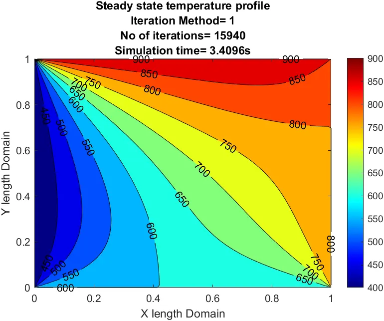
Plot for 2D heat conduction for Steady state using Jacobi Iterative method:

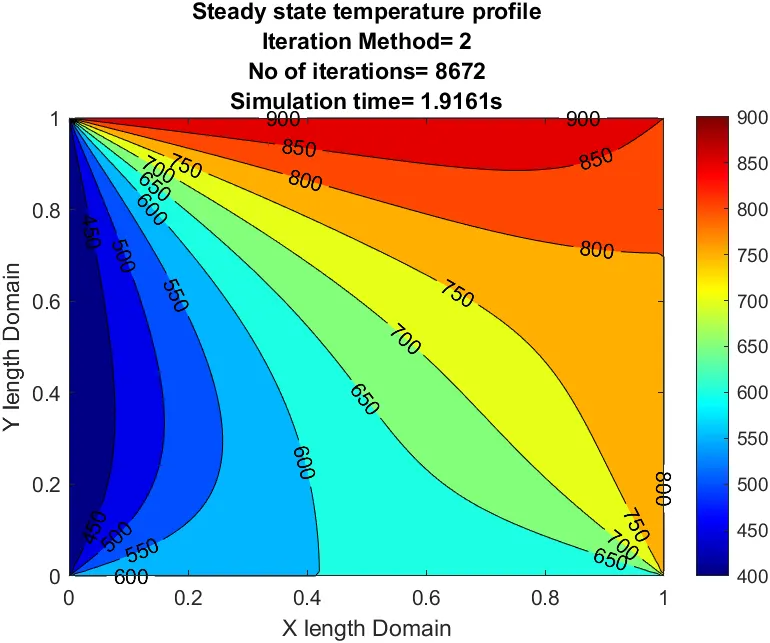
Plot for 2D heat conduction for Steady state using Gauss Siedel Iterative method:

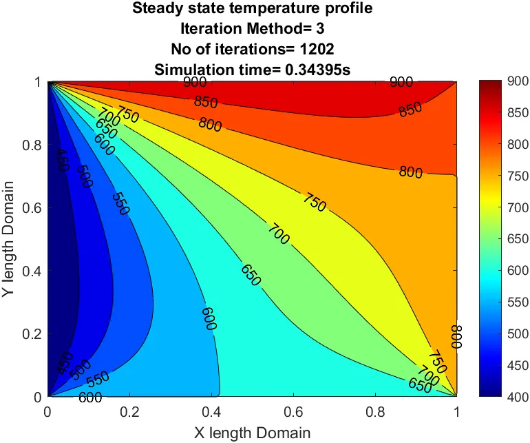
Plot for 2D heat conduction for Steady state using SOR Iterative method:

Solving 2D heat conduction equation for Unsteady state:

Governing equation for 2D heat conduction for unsteady state is

`(partialT)/(partialt)=alpha[(partial^2T)/(partialx^2)+(partial^2T)/(partialy^2)]` ............(2)

we need to solve above equation by using two scemes

• Explicit scheme
• Implicit scheme

Explicit scheme:

After applying first order forward differencing scheme on L.H.S and central differencing scheme on R.H.S on equation 2 , we get

`(Toverset(n+1)underset(i,j)()-Toverset(n)underset(i,j)())/(trianglet)=alpha[(Toverset(n)()underset(i+1,j)()-2Toverset(n)underset(i,j)()+Toverset(n)()underset(i-1,j)())/(trianglex^2)+(Toverset(n)()underset(i,j+1)()-2Toverset(n)()underset(i,j)()+Toverset(n)()underset(i,j-1)())/(triangley^2)]`

`Rightarrow Toverset(n+1)underset(i,j)()=Toverset(n)underset(i,j)()+alpha.trianglet[(Toverset(n)()underset(i+1,j)()-2Toverset(n)underset(i,j)()+Toverset(n)underset(i-1,j)())/(trianglex^2)+(Toverset(n)()underset(i,j+1)()-2Toverset(n)underset(i,j)()+Toverset(n)()underset(i,j-1)())/(triangley^2)]`

by assuming

`Toverset(n+1)underset(i,j)()=Toverset(n+1)underset(P)()`

`Toverset(n)underset(i,j)()=Toverset(n)underset(P)()`

`Toverset(n)underset(i+1,j)()=Toverset(n)underset(R)()`

`Toverset(n)underset(i-1,j)()=Toverset(n)underset(L)()`

`Toverset(n)underset(i,j+1)()=Toverset(n)underset(T)()`

`Toverset(n)underset(i,j-1)()=Toverset(n)underset(B)()`

And by simplification we get

`Toverset(n+1)underset(P)()=Toverset(n)underset(P)()(1-2kunderset(1)()-2kunderset(2)())+kunderset(1)()Toverset(n)underset(L)()+kunderset(1)()Toverset(n)underset(R)()+kunderset(2)()Toverset(n)underset(T)()+kunderset(2)()Toverset(n)underset(B)()`.............(3)

where k1 and k2 are

`kunderset(1)()=(alpha.trianglet)/(trianglex^2)`

`kunderset(2)()=(alpha.trianglet)/(triangley^2)`

Matlab code for Unsteady state 2D heat conduction profile in Explicit method:

clear all
close all
clc

l=1;
nx=60;
ny=nx;

%Defining space domain
x=linspace(0,1,nx);
dx=x(2)-x(1);
y=linspace(0,1,ny);
dy=y(2)-y(1);

%Calculation of time step
%dt=(0.5)/((alpha/dx^2)+(alpha/dy^2));
dt=0.00001;
alpha=1.4;

%Creating temperatures across given region
t=300*ones(nx,ny);
t(:,1)=400;
t(1,:)=600;
t(:,end)=800;
t(end,:)=900;

% %Temperature at edges
% t(1,1)=(600+400)/2;
% t(1,end)=(600+800)/2;
% t(end,1)=(400+900)/2;
% t(end,end)=(800+900)/2;

%Updating old t values
told=t;


CFL_num=(alpha*dt)*((1/dx^2)+1/(dy^2));


%Solving 2D unsteady state system
% [xx,yy]=meshgrid(x,y);
k1=(alpha*dt)/(dx^2);
k2=(alpha*dt)/(dy^2);

iter_method=1;

tic;
for k=1:7000
    for i =2:nx-1
        for j=2:ny-1
        term1=(1-2*k1-2*k2);
        term2=k1;
        term3=k2;
        H=(told(i-1,j)+told(i+1,j));
        V=(told(i,j-1)+told(i,j+1));
        t(i,j)=(told(i,j)*term1)+(term2*H)+(term3*V);
        end
    end
 told=t;
end
time=toc;
figure(1)
colormap(jet)
contourf(x,y,t,'showtext','on');
colorbar
% clabel(c,h);
title({'unsteady temperature profile';['Simulation time= ',num2str(time),'s']})
xlabel('X length Domian');
ylabel('Y length Domain');

Result:

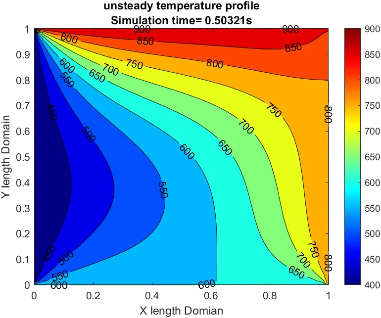
Plot for Unsteady state 2D heat conduction in Explicit method:

Implicit scheme:

Governing equation for 2D heat conduction for unsteady state is

`(partialT)/(partialt)=alpha[(partial^2T)/(partialx^2)+(partial^2T)/(partialy^2)]` ............(2)

After applying first order forward differencing scheme on L.H.S and central differencing scheme on R.H.S on equation 2 , we get

`(Toverset(n+1)underset(i,j)()-Toverset(n)underset(i,j)())/(trianglet)=alpha[(Toverset(n+1)underset(i+1,j)()-2Toverset(n+1)underset(i-1,j)()+Toverset(n+1)()underset(i-1,j)())/(trianglex^2)+(Toverset(n+1)underset(i,j+1)()-2Toverset(n+1)underset(i,j)()+Toverset(n+1)underset(i,j-1)())/(triangley^2)]`

`Rightarrow Toverset(n+1)underset(i,j)()=Toverset(n)underset(i,j)()+alpha.trianglet[(Toverset(n+1)underset(i+1,j)()-2Toverset(n+1)underset(i,j)()+Toverset(n+1)underset(i-1,j)())/(trianglex^2)+(Toverset(n+1)underset(i,j+1)()-2Toverset(n+1)underset(i,j)()+Toverset(n+1)underset(i,j-1)())/(triangley^2)]`

by assuming

`Toverset(n+1)underset(i,j)()=Toverset(n+1)underset(P)()`

`Toverset(n)underset(i,j)()=Toverset(n)underset(P)()`

`Toverset(n+1)underset(i+1,j)()=Toverset(n+1)underset(R)()`

`Toverset(n+1)underset(i-1,j)()=Toverset(n+1)underset(L)()`

`Toverset(n+1)underset(i,j+1)()=Toverset(n+1)underset(T)()`

`Toverset(n+1)underset(i,j-1)()=Toverset(n+1)underset(B)()`

And by simplification we get

`Toverset(n+1)underset(P)()(1+2kunderset(1)()+2kunderset(2)())=Toverset(n)underset(P)()+kunderset(1)()(Toverset(n+1)underset(L)()+Toverset(n+1)underset(R)())+kunderset(2)()(Toverset(n+1)underset(T)()+Toverset(n+1)underset(B)())`

where

`kunderset(1)()=(alpha.trianglet)/(trianglex^2)`

`kunderset(2)()=(alpha.trianglet)/(triangley^2`

`Toverset(n+1)underset(P)()=(Toverset(n)underset(P)()+kunderset(1)()(Toverset(n+1)underset(L)()+Toverset(n+1)underset(R)())+kunderset(2)()(Toverset(n+1)underset(T)()+Toverset(n+1)underset(B)()))/(1+2kunderset(1)()+2kunderset(2)()`

Matlab code for Unsteady state 2D heat conduction profile for Implicit method:

clear all
close all
clc

nx=50;
ny=50;

x=linspace(0,1,nx);
dx=1/(nx-1);
y=linspace(0,1,ny);
dy=1/(ny-1);

alpha=1.4;

%dt=(0.5)/((alpha/dx^2)+(alpha/dy^2));
dt=0.001;
tolerance=1e-4;
error=1e9;

t=300*ones(nx,ny);
t(:,1)=400;
t(1,:)=600;
t(:,end)=800;
t(end,:)=900;

%Temperature at edges
t(1,1)=(600+400)/2;
t(1,end)=(600+800)/2;
t(end,1)=(400+900)/2;
t(end,end)=(800+900)/2;

%Updating old t values
told=t;

CFL_num=(alpha*dt)*((1/dx^2)+1/(dy^2));

%Solving 2D steady state system

k1=(alpha*dt)/(dx^2);
k2=(alpha*dt)/(dy^2);

iter_method=input('Enter the iteration method number= ');
if iter_method==1
    %Computing Time loop
jacobi_iter=1;
for nt=1:600
    %Jacobi Iterative Solver
        tic
        term1=1/(1+2*k1+2*k2);
        term2=k1*term1;
        term3=k2*term1;
        error=1e9;
        while(error>tolerance)
            for i=2:nx-1
                for j=2:ny-1
                    H=(told(i-1,j)+told(i+1,j));
                    V=(told(i,j-1)+told(i,j+1));
                    t(i,j)=(told(i,j)*term1)+(term2*H)+(term3*V);
                end
            end
            error=max(max(abs(told-t)));
            told=t;
            jacobi_iter=jacobi_iter+1;
        end
        time1=toc;
end
end
  
    
%Gauss Siedel Iteration method

if iter_method==2
    gs_iter=1;
    tic
    for nt=1:600
        term1=1/(1+2*k1+2*k2);
        term2=k1*term1;
        term3=k2*term1;
        error=1e9;
        while(error>tolerance)
            for i=2:nx-1
            for j=2:ny-1
                H=(t(i-1,j)+told(i+1,j));
                V=(t(i,j-1)+told(i,j+1));
                t(i,j)=(told(i,j)*term1)+(term2*H)+(term3*V);
            end
            end
            error=max(max(abs(told-t)));
            told=t;
            gs_iter=gs_iter+1;
        end
        time2=toc;
    end
end



    
    %SOR iteration Mtehod
    omega=1.2;
    if iter_method==3
        sor_iter=1;
        tic
        for nt=1:600
        term1=1/(1+2*k1+2*k2);
        term2=k1*term1;
        term3=k2*term1;
        error=1e9;
        while(error>tolerance)
            for i=2:nx-1
                for j=2:ny-1
                    H=(t(i-1,j)+told(i+1,j));
                    V=(t(i,j-1)+told(i,j+1));
                    t(i,j)=(1-omega)*told(i,j)+omega*(term1*told(i,j)+term2*H+term3*V);
                end
            end
            error=max(max(abs(told-t)));
            told=t;
            sor_iter=sor_iter+1;
        end
        time3=toc;
        end
    end
    figure(1)
    [c,h]=contourf(x,y,t);
    clabel(c,h);
    colorbar;
    colormap(jet);
    
    if iter_method==1
        title({'Unsteady state temperature profile';['Iteration Method= Jacobi'];['No of iterations= ',num2str(jacobi_iter)]})
    elseif iter_method==2
        title({'Unsteady state temperature profile';['Iteration Method= Gauss Siedel'];['No of iterations= ',num2str(gs_iter)]})
    elseif iter_method==3
        title({'Unsteady state temperature profile';['Iteration Method= SOR'];['No of iterations= ',num2str(sor_iter)]})
    end

Result:

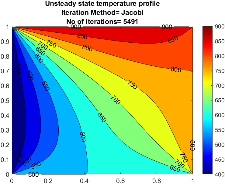
Plot for Unsteady state 2D heat conduction in Implicit method for Jacobi Iterations:

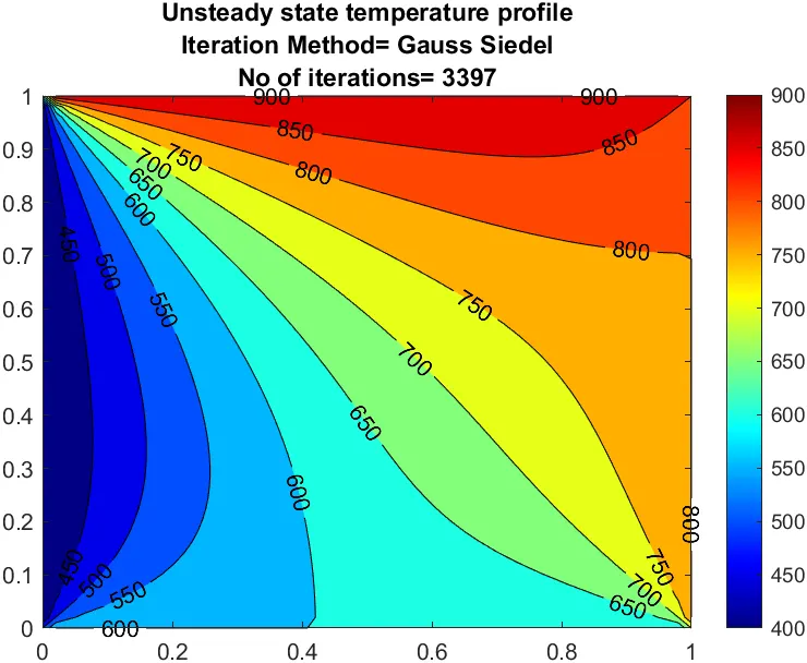
Plot for Unsteady state 2D heat conduction in Implicit method for Gauss Siedel Iterations:

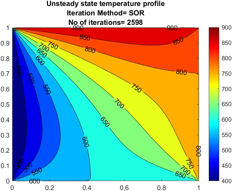
Plot for Unsteady state 2D heat conduction in Implicit method for SOR Iterations:

Conclusion and Explanation:

• Though we are getting same result for different iterative method so the difference between the no of iterations and computation time taken by iterative solver to get convergence result.
• By observing above plots it is clear that Jacobi iterations takes more than the other two iterative methods such as Gauss siedel and SOR .
• The computation time is also less in Jacobi iterations than other two iterative methods.
• The implicit method requires guess values and iterations for convergence as it is also based on the future state values. Which are not known at the time of computation. It checks convergence for each time step. This causes a delay in the simulation.
• Implicit method can be used to problems when converged results are nedded in less computation time as they are unconditionally stable. With increase in time step size the convergence rate is increased which leads to steady state with less no of itearations.
• Explicit method results time accurate solutions as it is governed by stability criteria in solution and when it is unstable it requires more no iterations.