Week 5.1 - Mid term project - Solving the steady and unsteady 2D heat conduction problem

2D Heat Conduction:

Heat conduction is defined as transfer of thermal energy within a medium from more energentic region to low energetic region.

The region in our case is a 2D plane and we will solve the Heat conduction equation for this region with a given boundary condition and for cases like steady case and unsteady case.

Governing Equations is given by:

`(delT)/(delt)+alpha_x(del^2T)/(delx^2)+alpha_y(del^2T)/(dely^2)=0` for unsteady 2D case

and `alpha_x(del^2T)/(delx^2)+alpha_y(del^2T)/(dely^2)=0` for steady 2D case.

We will solve the equation numerically instead of solving it analytically, as analytic solutions are not possible in most practical and complex cases.

But, before we can solve the above equations we have to discretize the above governing equations in algebric form. This is done using Taylor's series expansion. Looking at the unsteady case, the equation is parabolic in time and elliptical in space. Hence, using forward differencing in time and central differencing in space. whereas, looking at the steady case the corresponding equation is only eliptical in space and doesn't have any time term.

The discretization schemes we will be employing for steady and unsteady cases are :

1) Explicit schemes for Steady and Unsteady cases

In explicit scheme the dependent variable at the next time step is expressed as the values of the dependent variable at the previous time step explicitly.

Mathematically,

for unsteady state:

`[T_(i,j)^(n+1)-T_(i,j)^(n)]/(Deltat)=alpha_x{[T_(i+1,j)^n-2T_(i,j)^n+T_(i-1,j)^n]/(Deltax)^2}+alpha_y{[T_(i,j+1)^n-2T_(i,j)^n+T_(i,j-1)^n]/(Deltay)^2}`

which on simplification gives

`T_(i,j)^(n+1)=T_(i,j)^n+((alpha_xDeltat)/(Deltax^2))[T_(i+1,j)^n-2T_(i,j)^n+T_(i-1,j)^n]+((alpha_yDeltat)/(Deltay)^2)[T_(i,j+1)^n-2T_(i,j)^n+T_(i,j-1)^n]`

for steady state:

`T_(i,j)^n=1/2(1/(alpha_x/(Deltax)^2+(alpha_y)/(Deltay)^2])xx[alpha_x((T_(i+1,j)^n+T_(i-1,j)^n)/(Deltax)^2)+alpha_y((T_(i,j+1)^n+T_(i,j-1)^n)/(Deltay)^2)]`

though there is no time step in steady case and there is no explicit or implicit scheme for that matter but for most part it is similar to transient/unsteady explicit solver.The idea is to keep advancing the solution in time until the time-derivative vanishes. Explicit steady solvers try to use really large time-steps (acceleration) to speed this up.

2) Implicit Schemes for Unsteady case

In implicit scheme the dependent variable at next time step is expressed in terms of values of dependent variable at previous and next time step implicitly.

Mathematically,

`T_(i,j)^(n+1)=T_(i,j)^n+((alpha_xDeltat)/(Deltax^2))[T_(i+1,j)^(n+1)-2T_(i,j)^(n+1)+T_(i-1,j)^(n+1)]+((alpha_yDeltat)/(Deltay)^2)[T_(i,j+1)^(n+1)-2T_(i,j)^(n+1)+T_(i,j-1)^(n+1)]`

Explicit vs Implicit:

The advantage of explicit over implicit is that it is much faster than implicit but results are less accurate than the latter. Hence for simple and quick results Explicit is chosen over Implicit. However as the problem becomes more complex and accurate results are desired Implicit Scheme is the preferred choice.

For time variable we had Implicit schemes for grid spacing we have :

• Jacobi Iterations
• Gauss Seidel Iterations
• Successive Over-Relaxation (SOR)

Jacobi vs Gauss Seidel vs SOR:

In Jacobi Iterations we use previous iteration value to calculate values for next iterations.

In Gauss Seidel we use the updated values of the variable for the next iterations.

In SOR we over relaxed results from either of jacobi or gauss seidel for running iterations.

for eg. in steady case `T_(2,3)` is to be calculated, from steady state discrtized equation we get:

`T_(2,3)=1/2(1/(alpha_x/(Deltax)^2+(alpha_y)/(Deltay)^2])xx[alpha_x((T_(3,3)+T_(1,3))/(Deltax)^2)+alpha_y((T_(2,4)+T_(2,2))/(Deltay)^2)]`

In jacobi, all the temperature values on RHS will be of previous iteration or previously obtained temperature matrix.

In Gauss Seidel, updated values of `T_(1,3) and T_(2,2)` are used.

The Program has been divided into 2 main code sections:

1)Steady state analysis of 2D Heat conduction equation

%%
%Steady 2D heat conduction.
%since time derivative of Temperature vanishes the whold PDE reduces to
%d2T/dx2 + d2T/dy2 =0 which is elliptic in nature.
%This means the temperature at a given point is affected by temperature at
%neighbouring points and any disturbance is propagated in all direction at
%infinite speed.
%We will use explicit schemes for solving the steady case.
%We will use jacobi, Gauss_sidel and Succesive Over-relaxation methods to
%solve the steady state equation & compare the results and simulation time.
L=1;
nx_steady=15;
ny_steady=15;

[T_steady_jacobi,error_steady_jacobi,iter_jacobi]=steady_conduction_jacobi(nx_steady,ny_steady,L);

[T_steady_gs,error_steady_gs,iter_gs]=steady_conduction_gs(nx_steady,ny_steady,L);

[T_steady_sor,error_steady_sor,iter_sor]=steady_conduction_sor(nx_steady,ny_steady,L,T_steady_gs);

Above case solves steady state conduction using jacobi, gauss seidel and sor by calling respective functions:

1) Jacobi:

function [T_steady,error,iter]=steady_conduction_jacobi(nx_steady,ny_steady,L)
nx=nx_steady;                                                              %grid points in x direction
ny=ny_steady;                                                              %grid points in y direction
dx=L/nx;                                                                   %grid spacing in x direction
dy=L/ny;                                                                   %grid spacing in y direction

x=linspace(0,L,nx);
y=linspace(0,L,nx);
[xx,yy]=meshgrid(x,y);

T_initial=zeros(nx,ny);                                                    %Defining boundary conditions
T_initial(:,:)=700;                                                        %assumed temperature of inside grid points
T_initial(:,1)=400;                                                        %lHS face temperature
T_initial(:,ny)=800;                                                       %RHS face temperature
T_initial(1,:)=600;                                                        %TOP face temperature
T_initial(nx,:)=900;                                                       %BOTTOM face temperature
T_initial(1,1)=500;                                                        %TOP-LEFT corner temperature
T_initial(1,ny)=700;                                                       %TOP-RIGHT corner temperature 
T_initial(nx,ny)=850;                                                      %BOTTOM-RIGHT corner temperature
T_initial(nx,1)=650;                                                       %BOTTOM-LEFT corner temperature

T=T_initial;
T_old=T_initial;
error=9e9;
iter=0;

tic
while gt(error,1e-4)                                                       %converging loop
    iter=iter+1;
    for i=2:14                                                             %space iteration loop in x direction
        for j=2:14                                                         %space iteration llop in y direction
            term1=2*((dx^2)+(dy^2))/((dx^2)*(dy^2));
            term2=(T(i-1,j)+T(i+1,j))/(dx^2);
            term3=(T(i,j-1)+T(i,j+1))/(dy^2);
            T(i,j)=(term2+term3)/term1;
        end
    end
    error=max(max(abs(T-T_old)));                                          %error updation after space iterations
    T_old=T;
end
t=toc;

figure(1)
contourf(xx,yy,T,'ShowText','on')                                          %plotting results 
set(gca,'ydir','reverse')                                                  %reversing y axis
xlabel('x axis')
ylabel('y axis')
str=sprintf('2D Steady Conduction (Jacobi Method) \n Iterations = %d \n Computational Time = %f seconds',iter,t);
title(str)
colormap(jet)
colorbar
T_steady=T;
end

The code for gauss seidel and sor are similar with slight changes in logic-

2) Gauss Seidel:

tic
while gt(error,1e-4)                                                       %convergence loop
    iter=iter+1;
    for i=2:14                                                             %space iteration loop in x direction
        for j=2:14                                                         %space iteration loop in y direction
            term1=2*((dx^2)+(dy^2))/((dx^2)*(dy^2));
            term2=(T(i-1,j)+T(i+1,j))/(dx^2);
            term3=(T(i,j-1)+T(i,j+1))/(dy^2);
            T(i,j)=(term2+term3)/term1;
        end
    end
    error=max(max(abs(T-T_old)));                                          %error updation after space iterations
    T_old=T;
end
t=toc;

3) SOR:

tic
while gt(error,1e-4)                                                       %convergence loop
    iter=iter+1;
    for i=2:14                                                             %space iteration loop x direction
        for j=2:14                                                         %space iteration loop y direction
            T(i,j)=((1-a)*T_old(i,j))+(a*T_steady_gs(i,j));
        end
    end
    error=max(max(abs(T-T_old)));                                          %error updation after space iterations
    T_old=T;
end
t=toc;

2)Unsteady state analysis of 2D Heat Conduction Equation.

%%
%Unsteady 2D heat conduction equation.
%Governing PDE is given by (dT/dt)+ α(d2T/dx2 + d2T/dy2)=0.
%The equation is Parabolic in time and Eliptical in space.
%That means the disturbance will be marching ahead in time and in all
%direction in space.
%This code section plots for unsteady 2d conduction for both- explict and
%implicit cases; using jacobi, gauss seidel and SOR method.

nt=1500;
nx_unsteady=50;
ny_unsteady=50;
dt=1;
dx_unsteady=L/nx_unsteady;
dy_unsteady=L/ny_unsteady;

[T_unsteady_jacobi_exp,iter_unsteady_jacobi_exp]=unsteady_conduction_jacobi_exp(nt,nx_unsteady,ny_unsteady,dx_unsteady,dy_unsteady,dt);

[T_unsteady_gs_exp,iter_unsteady_gs_exp]=unsteady_conduction_gs_exp(nt,nx_unsteady,ny_unsteady,dx_unsteady,dy_unsteady,dt);

[T_unsteady_sor_exp,iter_unsteady_sor_exp]=unsteady_conduction_sor_exp(T_unsteady_gs_exp,nt,nx_unsteady,ny_unsteady,dx_unsteady,dy_unsteady,dt);

[T_unsteady_jacobi_imp,iter_unsteady_jacobi_imp]=unsteady_conduction_jacobi_imp(nt,nx_unsteady,ny_unsteady,dx_unsteady,dy_unsteady,dt);

[T_unsteady_gs_imp,iter_unsteady_gs_imp]=unsteady_conduction_gs_imp(nt,nx_unsteady,ny_unsteady,dx_unsteady,dy_unsteady,dt);

[T_unsteady_sor_imp,iter_unsteady_sor_imp]=unsteady_conduction_sor_imp(T_unsteady_gs_imp,nt,nx_unsteady,ny_unsteady,dx_unsteady,dy_unsteady,dt);

Above case solves unsteady state conduction using jacobi, gauss seidel and sor, explicitly and implicitly, by calling respective functions:

1) Jacobi

• Explicit

function [T_unsteady,iter]=unsteady_conduction_jacobi_exp(nt,nx_unsteady,ny_unsteady,dx_unsteady,dy_unsteady,dt)
nx=nx_unsteady;                                                            %grid points in x direction
ny=ny_unsteady;                                                            %grid points in y direction
dx=dx_unsteady;                                                            %grid spacing in x direction 
dy=dy_unsteady;                                                            %grid spacing in y direction

T_initial=zeros(nx,ny);                                                    %Defining initial conditions
T_initial(:,:)=100;                                                        %internal nodes temperatures
T_initial(:,1)=400;                                                        %LHS face temperature
T_initial(:,ny)=800;                                                       %RHS face temperature
T_initial(1,:)=600;                                                        %TOP face temperature
T_initial(nx,:)=900;                                                       %BOTTOM face temperatue
T_initial(1,1)=500;                                                        %TOP-LEFT corner temperature
T_initial(1,ny)=700;                                                       %TOP-RIGHT corner temperature
T_initial(nx,ny)=850;                                                      %BOTTOM-RIGHT corner temperature
T_initial(nx,1)=650;                                                       %BOTTOM-LEFT corner temperature

x=linspace(0,1,nx);
y=linspace(0,1,ny);
[xx,yy]=meshgrid(x,y);

alpha_x=1.88e-5;                                                           %Thermal diffusivity of STEEL
alpha_y=alpha_x;                                                           %considering ISOTROPIC nature of steel

cfl_x=((alpha_x)*(dt))/(dx^2);                                             %COURANT NUMBER in x direction
cfl_y=((alpha_y)*(dt))/(dy^2);                                             %COURANT NUMBER in y direction

T=T_initial;
T_old=T_initial;
iter=0;
cntr=0;

tic
figure(4)
for k=1:nt
    cntr=cntr+1;
    for i=2:nx-1
        for j=2:ny-1
            iter=iter+1;
            term1=(1-(2*cfl_x)-(2*cfl_y))*T_old(i,j);
            term2=(cfl_x)*(T_old(i+1,j)+T_old(i-1,j));
            term3=(cfl_y)*(T_old(i,j+1)+T_old(i,j-1));
            T(i,j)=term1+term2+term3;
        end   
    end
    T_old=T;
    contourf(xx,yy,T_old,'ShowText','on')                                  %plotting results
    set(gca,'ydir','reverse')                                              %reversing y axis
    xlabel('X axis');
    ylabel('Y axis');
    colormap(jet)
    colorbar
    str=sprintf('Unsteady 2D Conduction Jacobi Iteration (Explicit) \n Iterations %d \n CFL = %f',iter,cfl_x);
    title(str);
    pause(0.0001)
end
t=toc;
str=sprintf('Unsteady 2D Conduction Jacobi Iteration (Explicit) \n Iterations %d \n CFL = %f \n Commputational Time = %f seconds',iter,cfl_x,t);
title(str);
T_unsteady=T;
end

• Implicit:

Just 'for' loop changes rest remain the same.

figure(7)
tic
for k=1:nt                                                                 %time iteration loop
    error=9e9;
    while gt(error,1e-4)                                                   %convergence loop
          for i=2:nx-1                                                     %space iteration loop in x direction
              for j=2:ny-1                                                 %space iteration loop in y direction
                  iter=iter+1;
                  term1=T_previous(i,j);
                  term2=(cfl_x)*(T_old(i-1,j)+T_old(i+1,j));
                  term3=(cfl_y)*(T_old(i,j+1)+T_old(i,j-1));
                  term4=1+(2*cfl_x)+(2*cfl_y);
                  T(i,j)=(term1+term2+term3)/term4;
              end   
          end
          error=max(max(abs(T-T_old)));
          T_old=T;
    end
    T_previous=T;
    contourf(xx,yy,T_old,'ShowText','on')                                  %plotting results
    set(gca,'ydir','reverse')                                              %reversing y axis
    xlabel('X axis');
    ylabel('Y axis');
    colormap(jet)
    colorbar
    str=sprintf('Unsteady 2D Conduction Jacobi Iteration (Implicit) \n Iterations = %d \n CFL = %f',iter,cfl_x);
    title(str);
    pause(0.0001)
end
t=toc;

2)Gauss Seidel

• Explicit

figure(5)
tic
for k=1:nt
    cntr=cntr+1;
    for i=2:nx-1
        for j=2:ny-1
            iter=iter+1;
            term1=(1-(2*cfl_x)-(2*cfl_y))*T_old(i,j);
            term2=(cfl_x)*(T_old(i+1,j)+T(i-1,j));
            term3=(cfl_y)*(T_old(i,j+1)+T(i,j-1));
            T(i,j)=term1+term2+term3;
        end   
    end
    T_old=T;
    contourf(xx,yy,T_old,'ShowText','on')
    set(gca,'ydir','reverse')
    xlabel('X axis');
    ylabel('Y axis');
    colormap(jet)
    colorbar
    str=sprintf('Unsteady 2D Conduction Gauss Seidel Iteration (explicit) \n Iterations %d \n CFL = %f',iter,cfl_x);
    title(str);
    pause(0.0001)
end
t=toc;

• Implicit

figure(8)
tic
for k=1:nt                                                                 %time iteration loop
    error=9e9;                                          
    while gt(error,1e-4)                                                   %convergence loop
          for i=2:nx-1                                                     %space iteration loop in x direction
              for j=2:ny-1                                                 %space iteration loop in y direction
                  iter=iter+1;
                  term1=T_previous(i,j);
                  term2=(cfl_x)*(T(i-1,j)+T_old(i+1,j));
                  term3=(cfl_y)*(T_old(i,j+1)+T(i,j-1));
                  term4=1+(2*cfl_x)+(2*cfl_y);
                  T(i,j)=(term1+term2+term3)/term4;
              end   
          end
          error=max(max(abs(T-T_old)));
          T_old=T;
    end
    T_previous=T;
    contourf(xx,yy,T_old,'ShowText','on')                                  %plotting results
    set(gca,'ydir','reverse')                                              %reversing y axis
    xlabel('X axis');
    ylabel('Y axis');
    colormap(jet)
    colorbar
    str=sprintf('Unsteady 2D Conduction Gauss Seidel Iteration (Implicit) \n Iterations = %d \n CFL = %f',iter,cfl_x);
    title(str);
    pause(0.0001)
end
t=toc;

3)SOR

• Explicit

figure(6)
tic
for k=1:nt                                                                 %time iteration loop
    cntr=cntr+1;
    for i=2:nx-1                                                           %space iteration loop in x direction
        for j=2:ny-1                                                       %space ietration loop in y direction
            iter=iter+1;
            T(i,j)=((1-a)*T_old(i,j))+(a*T_unsteady_gs_exp(i,j));
        end   
    end
    T_old=T;
    contourf(xx,yy,T_old,'ShowText','on')                                  %plotting results
    set(gca,'ydir','reverse')                                              %reversing y axis
    xlabel('X axis');
    ylabel('Y axis');
    colormap(jet)
    colorbar
    str=sprintf('Unsteady 2D Conduction SOR Method (explicit)  \n Iterations %d \n CFL = %f',iter,cfl_x);
    title(str);
    pause(0.0001)
end
t=toc;

• Implicit

figure(9)
tic
for k=1:nt                                                                 %time iteration loop
    error=9e9;
    while gt(error,1e-4)                                                   %convergence loop
          for i=2:nx-1                                                     %space iteration loop in x direction
              for j=2:ny-1                                                 %space iteration loop in y direction
                  iter=iter+1;
                  T(i,j)=((1-a)*T_old(i,j))+(a*T_unsteady_gs_imp(i,j));
              end   
          end
          error=max(max(abs(T-T_old)));
          T_old=T;
    end
    contourf(xx,yy,T_old,'ShowText','on')                                  %plotting results
    set(gca,'ydir','reverse')                                              %reversing y axis
    xlabel('X axis');
    ylabel('Y axis');
    colormap(jet)
    colorbar
    str=sprintf('Unsteady 2D Conduction SOR Iteration (Implicit) \n Iterations = %d \n CFL = %f',iter,cfl_x);
    title(str);
    pause(0.0001)
end
t=toc;

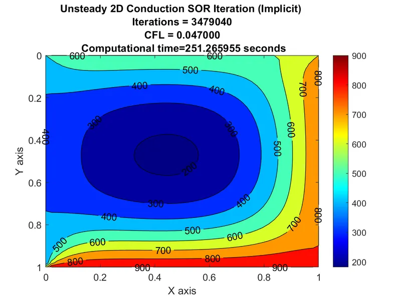
RESULT:

Following plots were obtained :

1)Steady Case:

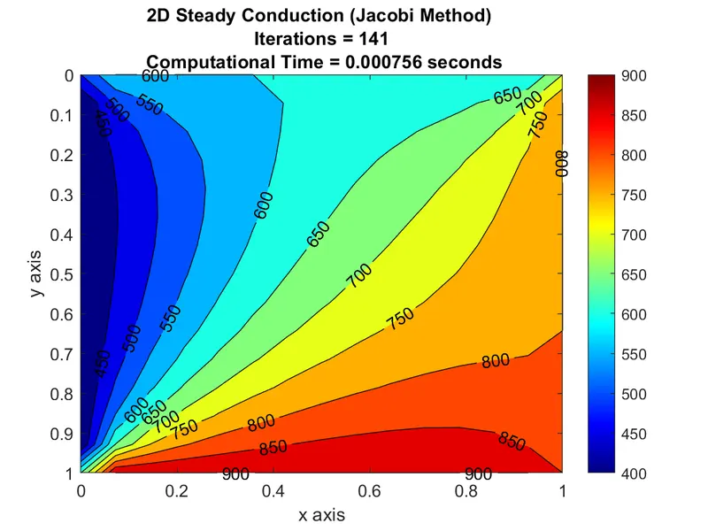
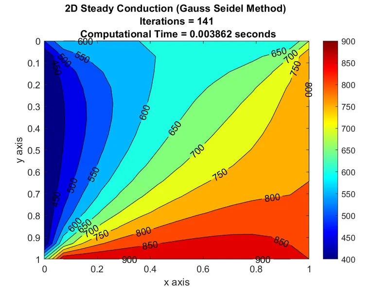
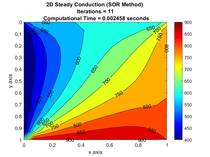
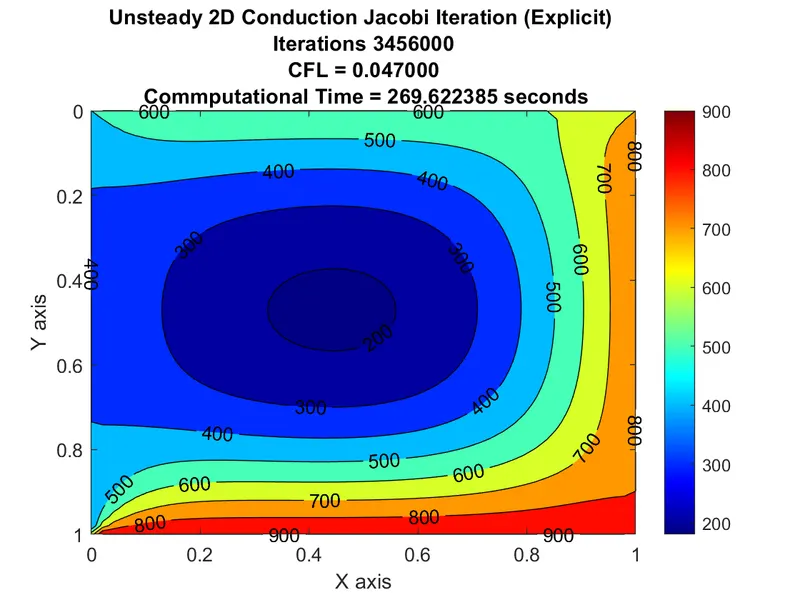
2) Unsteady case

a) Explicit Scheme

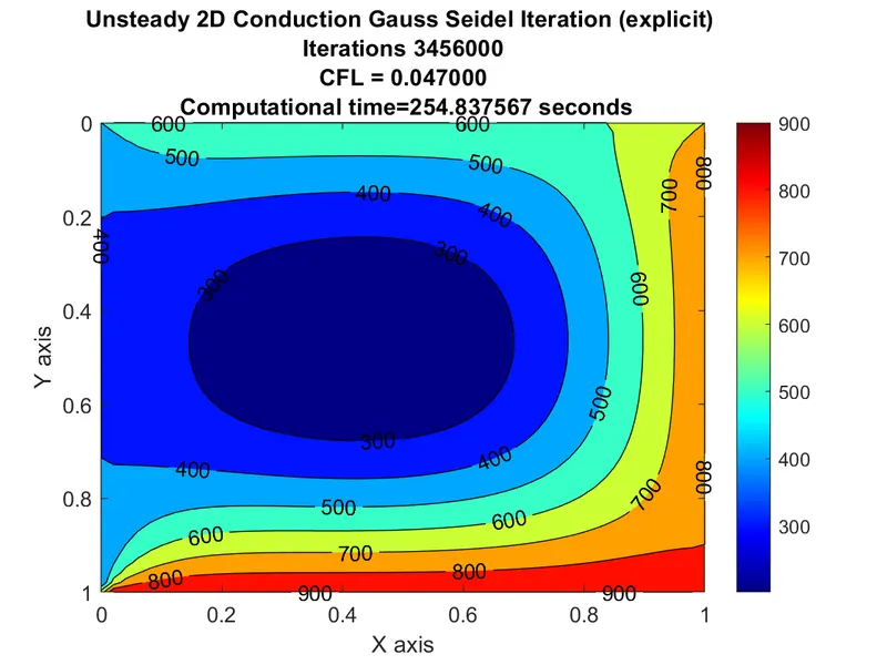
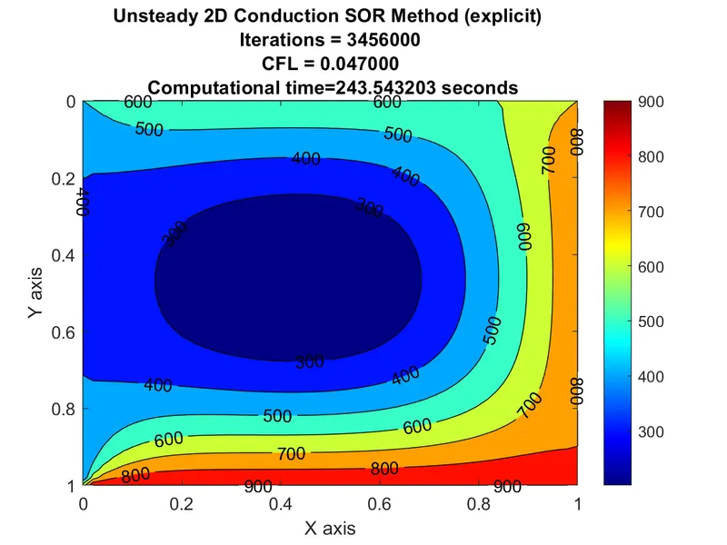
b) Implicit

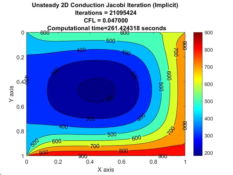
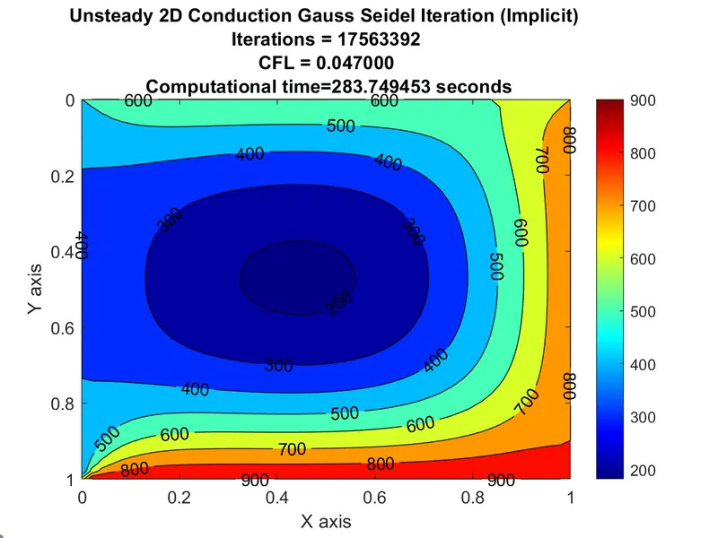
STEADY (EXPLICIT)	ITERATIONS	COMPUTATIONAL TIME (secs)
JACOBI	141	0.000756
GAUSS SEIDEL	141	0.003862
SOR	11	0.002458

UNSTEADY (EXPLICIT)	ITERATIONS	COMPUTATIONAL TIME (secs)
JACOBI	3456000	269.62
GAUSS SEIDEL	3456000	254.83
SOR	3456000	243.54

UNSTEADY (IMPLICIT)	ITERATIONS	COMPUTATIONAL TIME (secs)
JACOBI	21095424	261.42
GAUSS SEIDEL	17563392	283.74
SOR	3479040	251.26

CONCLUSION:

1) In Steady case, SOR gives the fastest result and converges in least number of iterations compared to jacobi and gauss seidel.

Also, `Iterations_(jacobi) >= Iterations_(gauss-seide l) >= Iterations_(SOR)`.

2) In Unsteady explicit method, number of iterations are same for jacobi, gauss seidel and SOR iterations which is still less than number of iterations of any of iterative techniques (jacbi, gauss seidel, SOR) of Implicit method.

i.e.: `Iterations_(ex plicit) < Iterations_(implicit)`

also unsteady case follows same trends as the steady case :

`Iterations_(jacobi) > Iterations_(gauss-seide l) > Iterations_(SOR)``

3) Computational time for Implicit Unsteady case is more than computational time for Explicit Unsteady case.

4)Explicit condtion limits the size of grid step for a given time step and vice versa. whereas there is no such condition for implicit case.

5)The computational time and number of iterations can also be reduced by selecting appropriate temperature in the domain. By appropriate temperature it is meant thant temperature values that are bounded by the domain conditions and type of problem being solved.