Week 5.1 - Mid term project - Solving the steady and unsteady 2D heat conduction problem

1)study state solver

clear all 
close all
 clc
 
 %initials
  l=1;%length of domin
  nx=100;
  ny=nx;
  
  x=linspace(0,l,nx);
  dx=x(2)-x(1);
  y=linspace(0,l,ny);
  dy=y(2)-y(1);
  
  %temperature values \ temperature matrix 
  t = 300*ones(ny,nx);
  t(:,1)=400;% temperature to left
  t(1,:)=600;% temperature at top 
  t(:,end)=800;% temperature to right 
  t(end,:)=900;% tempearture at bottom 
  
  %updateing the values of temp
  
  told = t;
  
  term=(dx^2*dy^2)/(2*(dx^2+dy^2));
  
  tolerance = 1e-4;
  error = 1e+8;
  
  iter_method = 1; % jacobi method 
  if iter_method == 1
          tic
          iter = 0;
          while(error>tolerance)
              for j=2:ny-1
                  for i=2:nx-1
                      t(i,j)=term*((told(i-1,j)+told(i+1,j))/(dx^2)+(told(i,j-1)+told(i,j+1))/(dy^2));
                  end 
              end 
              error  = max(max(abs(t-told)));
              told = t;
              iter= iter+1;
          end 
          time = toc;     
             
  elseif iter_method == 2 % gauss seidal method 
          tic;
          iter=0;
          while(error>tolerance)
              for j=2:ny-1
                  for i=2:nx-1
                      t(i,j)= term*(t(i-1,j)+told(i+1,j))/dx^2+(t(i,j-1)+told(i,j+1)/dy^2);
                  end 
              end
                  error = max(max(abs(t-told)));
                  told = t;
                  iter = iter+1;
          end 
             time = toc;
  elseif iter_method ==3 %sor method 
                  omega = 1.8;
                  tic 
                  iter = 0;
                  while (error>tolerance)
                      for j=2:ny-1
                          for i=2:nx-1
                              t(i,j) = term*((t(i-1,j)+told(i+1,j))/dx^2+(t(i,j-1)+told(i,j+1))/dy^2);
                              t(i,j)= told(i,j)*(1-omega)+(omega*t(i,j));
                          end
                      end 
                       error = max(max(abs(t-told)));
                      told=t;
                      iter = iter+1;
                  end 
                   time = toc;
  end 
             
  %plotting the results of temperature contour 
  [c,h] = contourf(x,y,t);
  clabel (c,h)
  colorbar
  colormap(jet)
  ax.YDir = 'reverse';
  xlabel('x_axis')
  ylabel('y_axis')
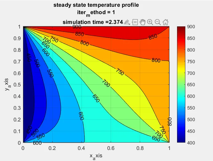
  title({'steady state temperature profile';['iter_method = ',num2str(iter_method)];['no. of iteration = ',num2str(iter)];['simulation time =',num2str(time),'s']})
  grid on 

results :- output for the iteration solver jacobi method

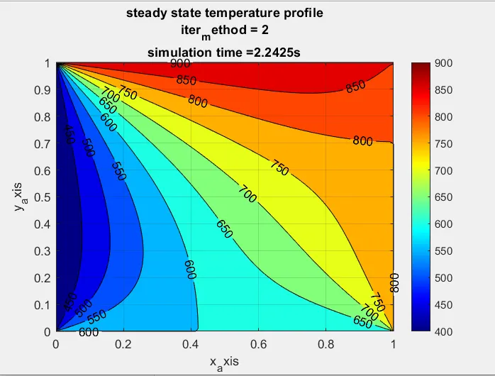
result:-output for iteration solver gauss seidal method

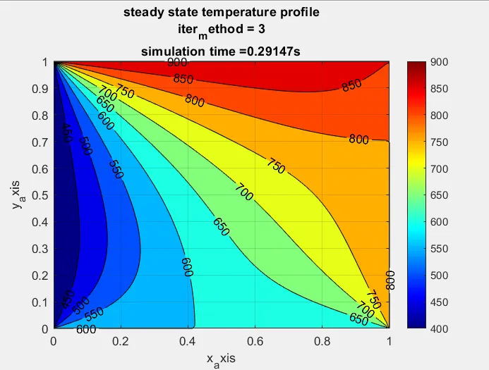
result:- output for iteartion of SOR method

explicit solver :-

clear all 
close all
clc

l=1;
nx=100;
ny=nx;
dt=0.14;
t=1000;%time step 
nt=t/dt;
alpha = 1.75e-4;

x=linspace(0,l,nx);
dx=x(2)-x(1);
y = linspace(0,l,ny);
dy=y(2)-y(1);
CFL=alpha*dt*((1/dx^2)+(1/dy^2));
%guess temperature matrix 
T=300*ones(ny,nx);
T(:,1)=400;%tepmerture to left 
T(1,:)=600; %temperture at top
T(:,end)=800;%temperture to right
T(end,:)=900;%temperature at bottom 
Told=T;%updateing the values of T
k1=alpha*dt/dx^2;
k2=alpha*dt/dy^2;

iter=0;
tic
%time loop
for k=1:nt
    %space loop for yaxis 
    for j=2:ny-1 
        for i=2:nx-1 %space loop for xaxis
            H=(Told(i-1,j)-2*Told(i,j)+Told(i+1,j));
            V=(Told(i,j-1)-2*Told(i,j)+Told(i,j+1));
            T(i,j)=Told(i,j)+(H*k1)+(V*k2);
        end 
    end 
    Told=T;
    iter = iter+1;
end 
time = toc;
%plotting for the temperature countour on x and Y axis 
[c,h] = contourf(x,y,T);
clabel(c,h);
colorbar
colormap(jet)
ax = gca;
ax.YDir = 'reverse';
xlabel('x')
ylabel('y')
title({'transient state-explicit temperature profile';['no.of iteration = ',num2str(iter),'Time=',num2str(t),'s'];['CFL=',num2str(CFL),'simulation time=',num2str(time)]})

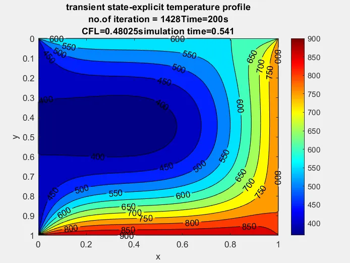
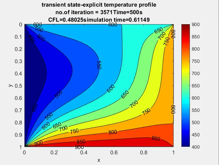
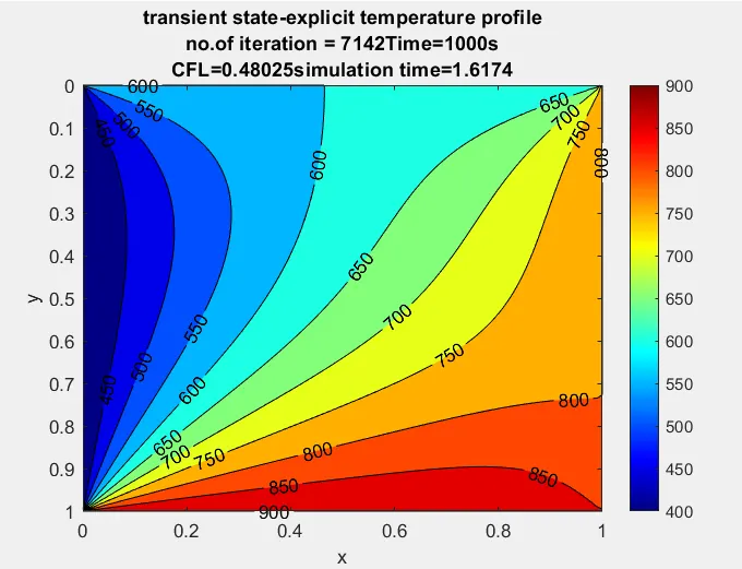
ploting the results of temperture profile for the time 200s,500s,and1000s

results1:- temperature profile for the time step 200s(explicite method )

result2:- temperature profile for the time 500s

result3:- temperature profile for the time 1000s

conclusion for explicite method :

1) temperature profile changes with the time

2) the temperature profile reaches stability state as the time goes on increases form 200s to 1000s,