Week 7 - Simulation of a 1D Super-sonic nozzle flow simulation using Macormack Method

1)program for solveing the 1-D super sonic nozzel flow using mackormac method (non-conservative form)

close all
clear all
clc
 n=30;
 L=3;
 x=linspace(0,L,n);
 dx=x(2)-x(1);
 gamma=1.4;
 rho=1-0.3146*x;
 T=1-0.2314*x;
 a=1+2.2*(x-1.5).^2;
 v=(0.1+1.09*x).*T.^0.5;
 m=v./(T.^0.5);
 mfr=rho.*a.*v;
 p=rho.*T;
%area

%time step
nt=1400;
dt=0.01;
%otput for time loop

for i=1:length(nt)
   nt=100; 
   rho_old=rho;
   T_old=T;
   v_old=v;
   for j=2:n-1
       %preductor step
       drho_dx=(rho(j+1)-rho(j))/dx;
       dv_dx=(v(j+1)-v(j))/dx;
       dT_dx=(T(j+1)-T(j))/dx;
       da_dx=(log(a(j+1))-log(a(j)))/dx;
       drho_dt_p(j)=-rho(j)*dv_dx-rho(j)*v(j)*da_dx-v(j)*drho_dx;
       dv_dt_p(j)=-v(j)*dv_dx-(1/gamma)*(dT_dx+(T(j)/rho(j)))*drho_dx;
       dT_dt_p(j)=-v(j)*dT_dx-(gamma-1)*T(j)*(dv_dx+v(j)*da_dx);
       %update the primitives
       v(j)=v_old(j)+dv_dt_p(j)*dt;
       rho(j)=rho_old(j)+drho_dt_p(j)*dt;
       T(j)=T_old(j)+dT_dt_p(j)*dt;
   end 
   for j=2:n-1
       %corrector method
       drho_dx=(rho(j)-rho(j-1))/dx;
       dv_dx=(v(j)-T(j-1))/dx;
       dT_dx=(T(j)-T(j-1))/dx;
       da_dx=(log(a(j))-log(a(j-1)))/dx;
       drho_dt_c(j)=-rho(j)*dv_dx-rho(j)*v(j)*da_dx-v(j)*drho_dx;
       dv_dt_c(j)=-v(j)*dv_dx-(1/gamma)*(dT_dx+(T(j)/rho(j)))*drho_dx;
       dT_dt_c(j)=-v(j)*dT_dx-(gamma-1)*T(j)*(dv_dx+v(j)*da_dx);
   end 
   
       %average timederivative
       drho_dt_avg=0.5*(drho_dt_p+drho_dt_c);
       dv_dt_avg=0.5*(dv_dt_p+dv_dt_c);
       dT_dt_avg=0.5*(dT_dt_p+dT_dt_c);
        %final correction values 
   for k=2:n-1
       rho(k)=rho_old(k)+drho_dt_avg(k)*dt;
       v(k)=v_old(k)+dv_dt_avg(k)*dt;
       T(k)=T_old(k)+dT_dt_avg(k)*dt;
   end 
       %entry bc
       v(1)=2*v(2)-v(3);
       %exit bc
       v(n)=2*v(n-1)-v(n-2);
        rho(n)=2*rho(n-1)-rho(n-2);
         T(n)=2*T(n-1)-T(n-2);
         %final update of primitives
         p=rho.*T;
         m=v./T.^0.5;
         error(k)=abs(v(k)-v(k-1));
         mfr=rho.*a.*v;
         
end 
 
     figure(1)
               plot(x,v,'b',x,p,'r',x,T,'k',x,rho,'m',x,m,'g',x,mfr,'c')
               ylim([-0.1 4])
               title(sprintf('time step=%d',i))
              xlabel('length of nozzel')
              ylabel('non dimensional parameters')
              legend('velocity','pressure','temperature','density','mach number','mass flow rate','location','northwest')
              title('non conseravtive form- steady state didtribution of primitive variables')     
  
                   
                   
      
       

result:-

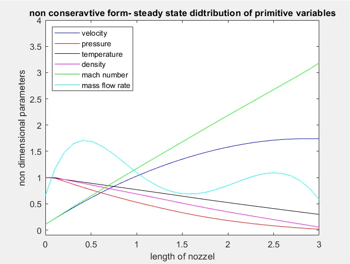
the above plot shows the behavior of the velocity,density,mach number,temperature,pressure and mass flow rate through the nozzel (non-conservative form)

2)program of solving the 1-D super sonicflow in nozzel (conservative form)

close all
clear all
clc

L=3;
n=31;
nt=150;
cfl=0.5;
x=linspace(0,L,n);
dx=x(2)-x(1);
gamma=1.4;
a=1+2.2*(x-1.5).^2;
for ii=1:length(x)
    if (x(ii)<=0.5)
        rho(ii)=1;
        T(ii)=1;
    elseif (x(ii)>0.5)&(x(ii)<=1.5)
        rho(ii)=1-0.366*(x(ii)-0.5);
        T(ii)=1-0.167*(x(ii)-0.5);
    elseif(x(ii)>1.5)&(x(ii)<=3.5)
        rho(ii)=0.634-0.3879*(x(ii)-1.5);
        T(ii)=0.833-0.3507*(x(ii)-1.5);
    end 
end       
 v=(0.1+1.09*x).*T.^0.5;
 m=v./(T.^0.5);
 mfr=rho.*a.*v;
 p=rho.*T;
 u1=rho.*a;
 u2=0.59*ones(1,n);
 u3=u1.*((T./(gamma-1))+(gamma/2).*v.^2);
 dt=0.01;
 
 for i=1:length(nt)
     %storing the old values 
     u1old=u1;
     u2old=u2;
     u3old=u3;
     
     for j=2:n-1
         f1=u2;
         f2=((u2.^2)./u1)+((gamma-1)/gamma)*(u3-((gamma/2)*(u2.^2)./u1));
         f3=((gamma.*u2.*u3)./u1)-((gamma*(gamma-1)/2)*(u2.^3)./(u1.^2));
         %source term
         j1=(1/gamma)*rho(j)*T(j)*((a(j+1)-a(j))/dx);
         %predictor step
         du1_dt_p(j)=-(f1(j+1)-f1(j))/dx;
         du2_dt_p(j)=-(f2(j+1)-f2(j))/dx+j1;
         du3_dt_p(j)=-(f3(j+1)-f3(j))/dx;
         %updateing the solution vector
         u1(j)=u1old(j)+du1_dt_p(j)*dt;
         u2(j)=u2old(j)+du2_dt_p(j)*dt;
         u3(j)=u3old(j)+du3_dt_p(j)*dt;
         %updateing the primitives 
         rho=u1./a;
         T=(gamma-1).*(u3./u1-(gamma/2).*(u2./u1).^2);
         %updateing the flux terms 
         f1=u2;
         f2=u2.^2./u1+((gamma-1)/gamma).*(u3-(gamma/2)*u2.^2./u1);
         f3=gamma.*u2.*u3./u1-0.5*gamma*(gamma-1).*u2.^3./u1.^2;
         %source term of correctior step
         j2=(1/gamma)*(rho(j)*T(j)*(a(j)-a(j-1))/dx);
         %corrector step
         du1_dt_c(j)=-(f1(j)-f1(j-1))/dx;
         du2_dt_c(j)=-(f2(j)-f2(j-1))/dx+j2;
         du3_dt_c(j)=-(f3(j)-f3(j-1))/dx;
     end 
     %average time derivatives
     du1_dt_avg=0.5*(du1_dt_p+du1_dt_c);
     du2_dt_avg=0.5*(du2_dt_p+du2_dt_c);
     du3_dt_avg=0.5*(du3_dt_p+du3_dt_c);
     %final corrector values 
     for k=2:n-1
         u1(k)=u1old(k)+du1_dt_avg(k)*dt;
         u2(k)=u2old(k)+du2_dt_avg(k)*dt;
         u3(k)=u3old(k)+du3_dt_avg(k)*dt;
     end 
     %entering bc
     u1(1)=a(1);
     u2(1)=2*u2(2)-u2(3);
     u3(1)=2*u3(n-1)-u3(n-2);
     %final update of primitives 
     rho=u1./a;
     v=u2./u1;
     T=(gamma-1).*(u3./u1-(gamma/2).*(u2./u1).^2);
     p=rho.*T;
     m=v./T.^0.5;
     error(k)=abs(v(k)-v(k-1));
     mfr=u2;
 end 
     
 
     figure(1)
               plot(x,v,'b',x,p,'r',x,T,'k',x,rho,'m',x,m,'g',x,mfr,'c')
               ylim([-0.1 4])
               title(sprintf('time step=%d',i))
              xlabel('length of nozzel')
              ylabel('non dimensional parameters')
              legend('velocity','pressure','temperature','density','mach number','mass flow rate','location','northwest')
              title('conseravtive form- steady state didtribution of primitive variables')     
  
     
         
 

result:-

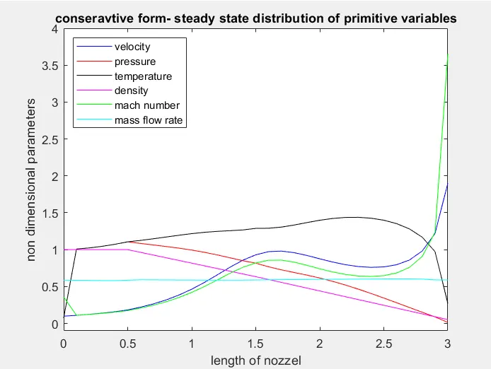
the above plot shows the behavior of the velocity,density,mach number,temperature,pressure and mass flow rate through the nozzel (conservative form)