Week 5.1 - Mid term project - Solving the steady and unsteady 2D heat conduction problem
Aim: - To write a program in MATLAB to solve a 2-D heat conduction equation by using point iterative techniques for steady and transient state.
Objective: -
- Solving the 2-D heat conduction equation for steady state and plot the temperature field analysis.
- Solving the 2-D heat conduction equation for transient state by implicit as well as explicit method and plot the temperature field after 5 sec.
- Solving the above two equation using following iterative techniques: -
- Jacobi
- Gauss-Seidel
- Successive Over-Relaxation.
Theory: -
Steady state 2-D heat conduction equation: - when the temperature of a field/region is not dependent on the time but only on the spatial co-ordinates, then it is called steady state. Its expression is as follows:
`(d^2 T)/(dx^2 ) +(d^2 T)/(dx^2 )=0`
Transient state 2-D heat conduction equation: - when the temperature of a region depends upon spatial co-ordinates as well as time also, then it is called transient state. Its expression is as follows:
`(dT)/dt+α( (d^2 T)/(dx^2 ) +(d^2 T)/(dx^2 ))=0`
here α is called thermal diffusivity.
To solve the equations the partial derivative terms are discretised by using forward differencing scheme for time derivative and central differencing scheme for spatial derivative. The discretised expression of terms are as follows -
`(dT)/dt=(T_(i,j)^(n+1)-T_(i,j)^n)/dt`
`(d^2 T)/(dx^2 )=(T_(i-1,j)-2T_(I,j)+T_(i+1,j))/(dx^2 )`
`(d^2 T)/(dy^2 )=(T_(i,j-1)-2T_(i,j)+T_(i,j+1))/(dy^2 )`
using the above expressions, we can formulate the expression for iterative techniques.
Methods of iteration
JACOBI: - In this method, the equations are solved by calculating the value of Temperature at inner nodes using several iterations, in which each value of temperature will be previously assigned temperature values at nodes.
GAUSS-SEIDEL – In this method, the 2D heat conduction equation solves, we are calculating the value of temperatures at inner nodes using several iterations, in which every value of temperature will be updated successively with respect to the previous iteration.
SUCCESSIVE OVER-RELAXATION- In this method, the 2D heat conduction equation solves. We are calculating the value of temperatures at inner nodes using several iterations, in which every value of temperature will be updated successively with respect to the previous iteration. And also “Relaxation factor” multiplies to the algebraic equation to alter the path of the iteration.
Expression obtained for different methods
Steady state -
Jacobi - `T_(i,j)=k1*(T_(i-1,j)+T_(i+1,j) )+k2*(T_(i,j-1)+T_(i,j+1))`
SOR - `T_(i,j)=(1-ω) T_(i,j)+ω(k1*(T_(i-1,j)+T_(i+1,j) )+k2*(T_(i,j-1)+T_(i,j+1) ))`
where `k1=(dy^2)/(2*(dx^2+dy^2 ))` and `k2=(dx^2)/(2*(dx^2+dy^2 ))`
Explicit Transient state -
Jacobi – `T_(i,j)^(n+1)=(1-2k1-2k2)*T_(i,j)^n+k1*(T_(i-1,j)^n+T_(i+1,j)^n )+k2*(T_(i,j-1)^n+T_(i,j+1)^n)`
SOR – `T_(i,j)^(n+1)=(1-ω) T_(i,j)^n+ω*((1-2k1-2k2)*T_(i,j)^n+k1*(T_(i-1,j)^n+ T_(i+1,j)^n )+k2*(T_(i,j-1)^n+T_(i,j+1)^n ))`
Here `k1=α*dt/(dx^2 )` and `k2=α*dt/(dy^2 )`
Implicit Transient state -
Jacobi– `T_(i,j)^(n+1)=(T_(i,j )^n+ k1*(T_(i-1,j)^n+T_(i+1,j)^n ) + k2*(T_(i,j-1)^n+T_(i,j+1)^n ))/(1+2k1+2k2)`
SOR - `T_(i,j)^(n+1)=(1-ω) T_(i,j)^n+ω*((T_(i,j )^n+ k1*(T_(i-1,j)^n+T_(i+1,j)^n ) + k2*(T_(i,j-1)^n+T_(i,j+1)^n ))/(1+2k1+2k2) )`
where `k1=α*dt/(dx^2 )` and `k2=α*dt/(dy^2 )`
The difference between Jacobi and Gauss seidel is only in the use of values of T. As in Jacobi the values used are all previous values, but in Gauss Seidel the value used are combination of calculated and previous values.
optimal value of `omega` can be calculate by `ω=2/(1+sin(πdx) )`
Given Values - Top boundary = 600 K
Bottom boundary = 900 K
Left boundary = 400 K
Right boundary = 800 K
Acceptable limit of error is 1e-4.
Simulation time for transient state is assumed to be 5 sec.
MATLAB code and their output: -
The code consists of one main program and 3 functions. Each section is provided with the output plot obtained by the functions:
Main program
close all
clear all
clc

l=1;
nx=41;
ny=41;
x=linspace(0,l,nx);
y=linspace(0,l,ny);
dx=x(2)-x(1);
dy=y(2)-y(1);
tol= 1e-4;
alpha=0.01 ;  %thermal diffusitivity for water at room temp in m^2/s

%initializing temperature field with room temp
T=300*ones(nx,ny);

%assigning given boundary temperature
T(:,1)= 400;
T(1,:)= 600;
T(:,end)= 800;
T(end,:)= 900;

%refining corner temperature
T(1,1) = (400+600)/2;
T(1,end)= (600+800)/2;
T(end,1)= (900+400)/2;
T(end,end)= (800+900)/2;

[xx,yy]=meshgrid(x,y);
%initial temperature field
p=figure(1);
[c,h]=contourf(xx,yy,T);
colorbar;
colormap(jet);
title('initial temperature field');
xlabel('X domain');
ylabel('Y domain');
set(p,'Visible','on')

%calling steady state function
steadystate(nx,ny,x,y,dx,dy,T,tol);

%calling explicit transient state function
explict_transient(nx,ny,x,y,dx,dy,T,tol);

%calling implicit transient state function
implict_transient(nx,ny,x,y,dx,dy,T,tol);
Output -
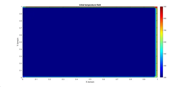
Function for steady state analysis
%steady state anlysis
function [] = steadystate(nx,ny,x,y,dx,dy,T,tol)

[xx,yy]=meshgrid(x,y);
T1=T;
Told= T1;
%calculating the value of constant
k1= (dy^2)/(2*((dx^2)+ (dy^2)));
k2= (dx^2)/(2*((dx^2)+ (dy^2)));
 for iterative_solver = [1,2,3]
%% jacobi steady state
  if iterative_solver ==1
      %initialising counter and error value
      jcntr=0;
      error=9e9;
 tic % starting the timer
    while (error>tol)  % loop termination condition
     for i=2:ny-1
         for j=2:nx-1
             T(i,j)= k1*(Told(i-1,j)+Told(i+1,j))+k2*(Told(i,j-1)+Told(i,j+1));
         end
     end
     %finding maximum error
     error= max(max(abs(Told-T)));
     %updating Told values with new calculated T values
     Told=T;
     jcntr=jcntr+1;
    end
    a=toc;
    %plotting the values
    figure(2)
   [c,h]=contourf(xx,yy,T);
   set(gca,'Ydir','reverse');
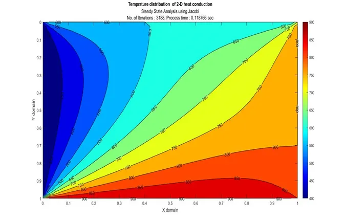
   title_text=sprintf('Steady State Analysis using JacobinNo. of Iterations : %.0f, Process time : %f sec',jcntr,a);
   title('Temprature distribution  of 2-D heat conduction', title_text);
   colormap(jet);
   colorbar;
   clabel(c,h);
   xlabel('X domain');
   ylabel('Y domain');

  end
 %% gauss siedel steady state
  if iterative_solver ==2
      %reinitializing the Told value with original initial temp field
      Told=T1;
      %initialising the counter and error
      gscntr=0;
      error=9e9;
 tic
    while (error>tol)  % loop termination condition
     for j=2:ny-1
         for i=2:nx-1
             T(i,j)= k1*(T(i-1,j)+Told(i+1,j))+k2*(T(i,j-1)+Told(i,j+1));
         end
     end
     error= max(max(abs(Told-T)));
     %updating Told values with new calculated T values
     Told=T;
     gscntr=gscntr+1;
    end
    a=toc;
    %plotting the values
    figure(3)
   [c,h]=contourf(xx,yy,T);
   set(gca,'Ydir','reverse');
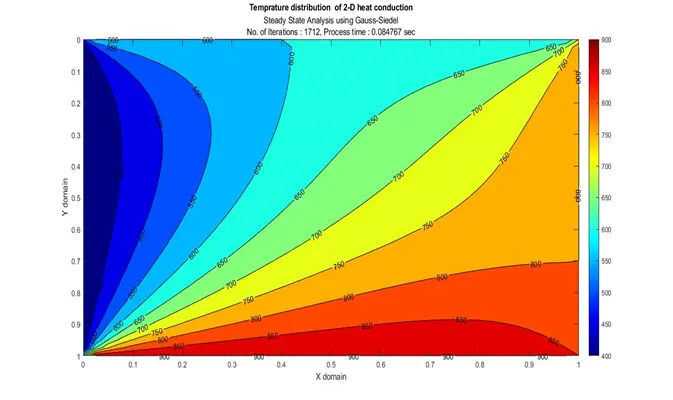
   title_text=sprintf('Steady State Analysis using Gauss-SiedelnNo. of Iterations : %.0f, Process time : %f sec',gscntr,a);
   title('Temprature distribution  of 2-D heat conduction', title_text);
   colormap(jet);
   colorbar;
   clabel(c,h);
   xlabel('X domain');
   ylabel('Y domain');

  end
  %% SOR steady state
  if iterative_solver ==3
   %reinitializing the Told value with original initial temp field
      Told=T1;
   %initialising the counter and error and omega value
      error=9e9;
      sorcntr=0;
      omega=1.4;
 tic
    while (error>tol)     % loop termination condition
     for j=2:ny-1
         for i=2:nx-1
             T(i,j)= Told(i,j)*(1-omega)+(k1*(T(i-1,j)+Told(i+1,j))+k2*(T(i,j-1)+Told(i,j+1)))*omega;
         end
     end
     error= max(max(abs(Told-T)));
       %updating Told values with new calculated T values
     Told=T;
     sorcntr=sorcntr+1;
    end
    a=toc;
    %plotting the values
    figure(4)
  [c,h]=contourf(xx,yy,T);
  set(gca,'Ydir','reverse');
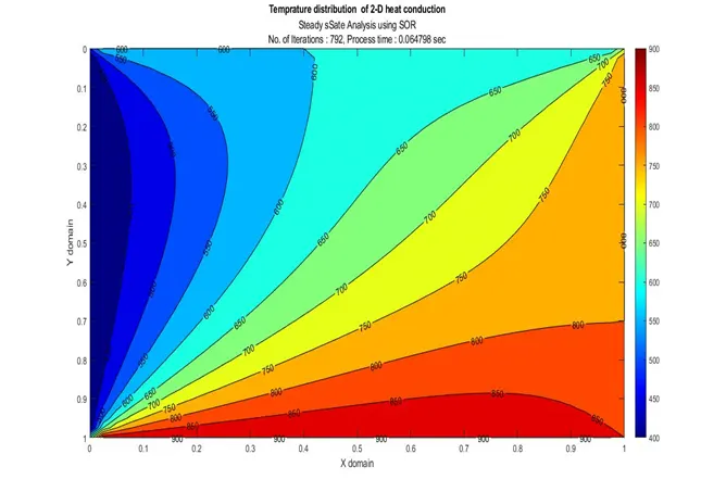
   title_text=sprintf('Steady sSate Analysis using SORnNo. of Iterations : %.0f, Process time : %f sec',sorcntr,a);
   title('Temprature distribution  of 2-D heat conduction', title_text);
   colormap(jet);
   colorbar;
   clabel(c,h);
   xlabel('X domain');
   ylabel('Y domain');

 end
 end
end
Output: -
- jacobi
2. Gauss-Seidel
3. SOR
function for Explicit transient state
% Transient state analysis by explicit method
function []=explict_transient(nx,ny,x,y,dx,dy,T,tol)

[xx,yy]=meshgrid(x,y);
T1=T;
Told= T;
Tprev=T;
alpha=.01;
simt=5;
t=linspace(0,simt,1500);
dt=t(2)-t(1);

%calculating the value of constant
k1= alpha*(dt/((dx)^2));
k2= alpha*(dt/((dy)^2));
for iterative_solver = [1,2,3]
%% JACOBI EXPLICIT
  if iterative_solver ==1
      jcntr=0;
 tic
 for k=1:length(t) %time loop
     error=9e9;
    while (error>tol)
     for j=2:ny-1
         for i=2:nx-1
             H = Told(i-1,j) + Told(i+1,j);
             V = Told(i,j-1) + Told(i,j+1);
             T(i,j)= (1-2*k1 - 2*k2)*Tprev(i,j) + (k1*H) + (k2*V);
         end
     end
     error= max(max(abs(Told-T)));
     %updating Told values with new calculated T values
     Told=T;
     jcntr=jcntr+1;
    end
     %updating Tprev value after every time loop run
     Tprev=T;
 end
    a=toc;
    % plotting the values
    figure(5)
   [c,h]=contourf(xx,yy,T);
   set(gca,'Ydir','reverse');
   title_text=sprintf('Transient State Analysis using Explicit JacobinNo. of Iterations : %.0f, Process time : %f sec',jcntr,a);
   title('Temprature distribution  of 2-D heat conduction', title_text);
   colormap(jet);
   colorbar;
   clabel(c,h);
   xlabel('X domain');
   ylabel('Y domain');

  end
  %% GAUSS SIEDEL EXPLICIT
  if iterative_solver == 2
      gscntr=0;
      %reinitializing the Told and Tprev value with original initial temp field
      Told=T1;
      Tprev=T1;
       tic
 for k=1:length(t)
     error=9e9;
    while (error>tol)
     for j=2:ny-1
         for i=2:nx-1
             H = T(i-1,j) + Told(i+1,j);
             V = T(i,j-1) + Told(i,j+1);
             T(i,j)= (1-2*k1 - 2*k2)*Tprev(i,j) + (k1*H) + (k2*V);
         end
     end
     error= max(max(abs(Told-T)));
     %updating Told values with new calculated T values
     Told=T;
     gscntr=gscntr+1;
    end
    %updating Tprev value after every time loop run
     Tprev=T;
 end
    a=toc;

   % plotting the values
    figure(6)
   [c,h]=contourf(xx,yy,T);
   set(gca,'Ydir','reverse');
   title_text=sprintf('Transient State Analysis using Explicit Gauss-SiedelnNo. of Iterations : %.0f, Process time : %f sec',gscntr,a);
   title('Temprature distribution  of 2-D heat conduction', title_text);
   colormap(jet);
   colorbar;
   clabel(c,h);
   xlabel('X domain');
   ylabel('Y domain');

  end

  %% SOR EXPLICIT
   if iterative_solver == 3
       omega=1.1;       % assigining the value of omega
       sorcntr=0;
 %reinitializing the Told and Tprev value with original initial temp field
      Told=T1;
      Tprev=T1;
       tic
 for k=1:length(t)
     error=9e9;
    while (error>tol)
     for j=2:ny-1
         for i=2:nx-1
             H = T(i-1,j) + Told(i+1,j);
             V = T(i,j-1) + Told(i,j+1);
             T(i,j)=((1-omega)*Told(i,j))+(omega*(((1-2*k1-2*k2)*Tprev(i,j))+(k1*H)+(k2*V)));
         end
     end
     error= max(max(abs(Told-T)));
     %updating Told values with new calculated T values
     Told=T;
     sorcntr=sorcntr+1;
    end
   %updating Tprev value after every time loop run
     Tprev=T;
 end
    a=toc;

    %plotting the values
    figure(7)
   [c,h]=contourf(xx,yy,T);
   set(gca,'Ydir','reverse');
   title_text=sprintf('Transient State Analysis using Explicit SORnNo. of Iterations : %.0f, Process time : %f sec',sorcntr,a);
   title('Temprature distribution  of 2-D heat conduction', title_text);
   colormap(jet);
   colorbar;
   clabel(c,h);
   xlabel('X domain');
   ylabel('Y domain');

  end


end
end
Output: -
1. Jacobi explicit
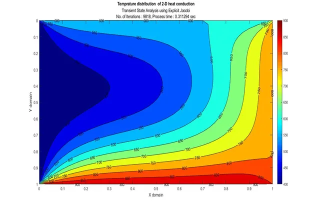
2. Gauss-Seidel explicit
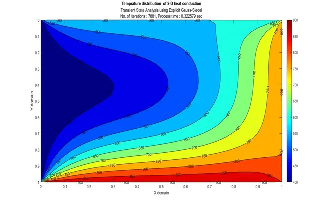
3. SOR
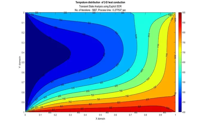
function for Implicit transient state
% Transient state analysis by implicit method
function [T_ijac,T_igs,T_isor,ai,icntr,cfl_iu]=implict_transient(nx,ny,x,y,dx,dy,T,tol)

[xx,yy]=meshgrid(x,y);
T1=T;
Told= T;
Tprev=T;
alpha=.01;
simt=5;
t=linspace(0,simt,1500);
dt=t(2)-t(1);

%calculating the value of constant
k1= alpha*(dt/((dx)^2));
k2= alpha*(dt/((dy)^2));
cfl_iu=k1+k2;

%%
%JACOBI IMPLICIT

      jcntr=0;
 tic
 for k=1:length(t) %time loop
     error=9e9;
    while (error>tol)
     for j=2:ny-1
         for i=2:nx-1
             H = Told(i-1,j) + Told(i+1,j);
             V = Told(i,j-1) + Told(i,j+1);
             T(i,j)= (Tprev(i,j)+(k1*H) + (k2*V))/(1+2*k1+2*k2);
         end
     end
     error= max(max(abs(Told-T)));
      %updating Told values with new calculated T values
     Told=T;
     jcntr=jcntr+1;
    end
     %updating Tprev value after every time loop run
     Tprev=T;
 end
 T_ijac=T;
    a_ijac=toc;
     figure(8)
   [c,h]=contourf(xx,yy,T);
   set(gca,'Ydir','reverse');
   title_text=sprintf('Transient State Analysis using Implicit Jacobi\nNo. of Iterations : %.0f, Process time : %f sec',jcntr,a_ijac);
   title('Temprature distribution  of 2-D heat conduction', title_text);
   colormap(jet);
   colorbar;
   clabel(c,h);
   xlabel('X domain');
   ylabel('Y domain');


  %%
  %GAUSS SIEDEL IMPLICIT

      gscntr=0;
      %reinitializing the Told and Tprev value with original initial temp field
      Told=T1;
      Tprev=T1;
       tic
 for k=1:length(t)
     error=9e9;
    while (error>tol)
     for j=2:ny-1
         for i=2:nx-1
             H = T(i-1,j) + Told(i+1,j);
             V = T(i,j-1) + Told(i,j+1);
              T(i,j)= (Tprev(i,j)+(k1*H) + (k2*V))/(1+2*k1+2*k2);
         end
     end
     error= max(max(abs(Told-T)));
      %updating Told values with new calculated T values
     Told=T;
     gscntr=gscntr+1;
    end
     %updating Tprev value after every time loop run
     Tprev=T;
 end
 T_igs=T;
    a_igs=toc;

    figure(9)
   [c,h]=contourf(xx,yy,T);
   set(gca,'Ydir','reverse');
   title_text=sprintf('Transient State Analysis using Implicit Gauss-Siedel\nNo. of Iterations : %.0f, Process time : %f sec',gscntr,a_igs);
   title('Temprature distribution  of 2-D heat conduction', title_text);
   colormap(jet);
   colorbar;
   clabel(c,h);
   xlabel('X domain');
   ylabel('Y domain');


  %%
  %SOR IMPLICI
       omega=1.08;    % assigining the value of omega
      sorcntr=0;
  %reinitializing the Told and Tprev value with original initial temp field
      Told=T1;
      Tprev=T1;
       tic
 for k=1:length(t)
     error=9e9;
    while (error>tol)
     for j=2:ny-1
         for i=2:nx-1
             H = T(i-1,j) + Told(i+1,j);
             V = T(i,j-1) + Told(i,j+1);
             T(i,j)=((1-omega)*Told(i,j))+(omega*((Tprev(i,j))+(k1*H)+(k2*V))/(1+2*k1+2*k2));
         end
     end
     error= max(max(abs(Told-T)));
    %updating Told values with new calculated T values
     Told=T;
     sorcntr=sorcntr+1;
    end
  %updating Tprev value after every time loop run
     Tprev=T;
 end
 T_isor=T;
    a_isor=toc;

    figure(10)
   [c,h]=contourf(xx,yy,T);
   set(gca,'Ydir','reverse');
    title_text=sprintf('Transient State Analysis using Implicit SOR\nNo. of Iterations : %.0f, Process time : %f sec',sorcntr,a_isor);
   title('Temprature distribution  of 2-D heat conduction', title_text);
   colormap(jet);
   colorbar;
   clabel(c,h);
   xlabel('X domain');
   ylabel('Y domain');


 icntr=[jcntr,gscntr,sorcntr];
 ai=[a_ijac,a_igs,a_isor];
end
Output: -
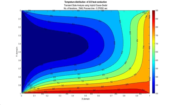
1. Jacobi implicit
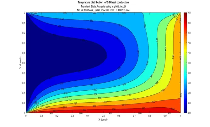
2. Gauss-Seidel implicit
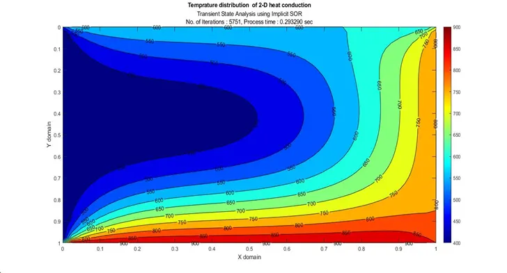
3.SOR
Conclusion: -
- Number of iterations for the methods are as follows for all three types of equations in descending order are -
Jacobi > Gauss- Seidel > Successive Over relaxation
- Even though no. of iteration is less but solving time is sometime greater than other due to complexity of the solution such as in implicit SOR iteration is less than Gauss-seidel but still the process time is a fraction more.
- Jacobi is relatively simpler than gauss-seidel and SOR in formulation.
- SOR largely depends on `ω` as selecting appropriate value can converge faster but if wrong it can over shoot the right value and tend to oscillate hence more no of iterations.