Challenge

Solving the steady and unsteady 2D heat conduction problem

SSuleman Ansari2 Nov 2021

AIM: The aim of this project is to solve steady and unsteady 2D heat conduction equation.

THEORY: The heat conduction equation is a partial differential equation that describes the distribution of heat (or the temperature field) in a given body over time.

Assumption & Boundary conditions to solve the steady and unsteady equation:

Assuming that the domain is a unit square.
Assuming that nx = ny (Number of points along the x direction is equal to the number of points along the y direction).
Boundary conditions for steady and unsteady case.
Left:400K
Top:600K
Right:800K
Bottom:900K
Tolerance=1e-4

Govering equation for 2D heat conduction equation for steady state

`(del^2T)/(delx^2)+(del^2T)/(dely^2)=0`

SOLVING 2D HEAT CONDUCTION EQUATION FOR STEADY STATE:

Discretize the equation by using central differencing scheme

`((T^n)_(i+1,j) -(2T^n)_(i,j)+(T^n)_(i-1,j))/(Deltax^2)+((T^n)_(i,j+1) -(2T^n)_(i,j)+(T^n)_(i,j-1))/(Deltay^2)=0`

`(T^n)_(i,j)=1/K[((T^n)_(i+1,j)+(T^n)_(i-1,j))/(Deltax^2)+((T^n)_(i,j+1)+(T^n)_(i,j-1))/(Deltay^2)]`

where k : `K=2[(Deltax^2+Deltay^2)/(Deltax^2.Deltay^2)]`

MAIN CODE 1:

%Solving the steady 2D heat conduction equation
clear all
close all
clc

%Inputs
nx=40; %no of grids-x-direction
ny=40; %no of grids-y-direction
rf=1.5;%relexation factor

%Calculation
x=linspace(0,1,nx);
y=linspace(0,1,ny);
dx=x(2)-x(1); %Time step-x-direction
dy=y(2)-y(1); %Time step-y-direction

%Assigning BC
T=ones(nx,ny);
T(1,:)=600;   %Top Boundary
T(end,:)=900; %Bottom Boundary
T(:,1)=400;   %Left Boundary
T(:,end)=800; %Right Boundary

Told=T;

%Constant
K=2*((dx^2+dy^2)/(dx^2*dy^2));
error=1;  %error
tol=1e-4; %tolerance

iterative_solver=input('enter iterative solver=')

%Jacobi Method
tic
if iterative_solver==1;
  jacobi_iter=1;
  while (error>tol)
  
        for i=2:nx-1
        for j=2:ny-1
            A=(Told(i-1,j)+Told(i+1,j))/(dx^2);
            B=(Told(i,j-1)+Told(i,j+1))/(dy^2);
            T(i,j)=(A+B)/K;
        
        end
        end
            error=max(max(abs(Told-T)));
            Told=T;
            jacobi_iter=jacobi_iter+1;

  end

     time1=toc;
     figure(1)
     colormap(jet)
     contourf(x,y,T,':','showText','on')
     xlabel('X axis')
     ylabel('Y axis')
     set(gca,'YDIR','reverse');
     text1=sprintf('Number of iteration= %d',jacobi_iter);
     text2=sprintf('Simulation time=%d s',time1);
     title(['Jacobi Solver Steady State';text1;text2]);
     colorbar
     pause(0.3)
end

%Gauss seidal Method
tic 
if iterative_solver==2
   gs_iter=1;
   while(error>tol)
          for i=2:nx-1
          for j=2:ny-1
              A=(T(i-1,j)+Told(i+1,j))/dx^2;
              B=(T(i,j-1)+Told(i,j+1))/dy^2;
              T(i,j)=(A+B)/K;
          end
          end
              error=max(max((abs(Told-T))));
              Told=T;
              gs_iter=gs_iter+1;
   end

       time2=toc;
       figure(2)
       colormap(jet)
       contourf(x,y,T,'showText','on')
       xlabel('X axis')
       ylabel('Y axis')
       set(gca,'YDIR','reverse');
       text1=sprintf('Number of iteration= %d',gs_iter);
       text2=sprintf('Simulation time=%d s',time2);
       title(['Gauss seidal Steady state';text1;text2]);
       colorbar
       pause(0.03)
end

%SOR Method
tic
if iterative_solver==3
   sor_iter=1;
    while(error>tol)
        for i=2:nx-1
        for j=2:ny-1
            A=(T(i-1,j)+Told(i+1,j))/dx^2;
            B=(T(i,j-1)+Told(i,j+1))/dy^2;
            T(i,j)=Told(i,j)*(1-rf)+rf*((A+B)/K);
        end
        end
           error=max(max(abs(Told-T)));
           Told=T;
           sor_iter=sor_iter+1;
    end
           time3=toc;
           figure(3)
           colormap(jet)
           contourf(x,y,T,'showText','on')
           xlabel('X axis')
           ylabel('Y axis')
           set(gca,'YDIR','reverse');
           text1=sprintf('Number of iteration= %d',sor_iter);
           text2=sprintf('Simulation time=%d s',time3);
           title(['SOR Steady state';text1;text2]);
           colorbar
           pause(0.03)
end

RESULTS 1:

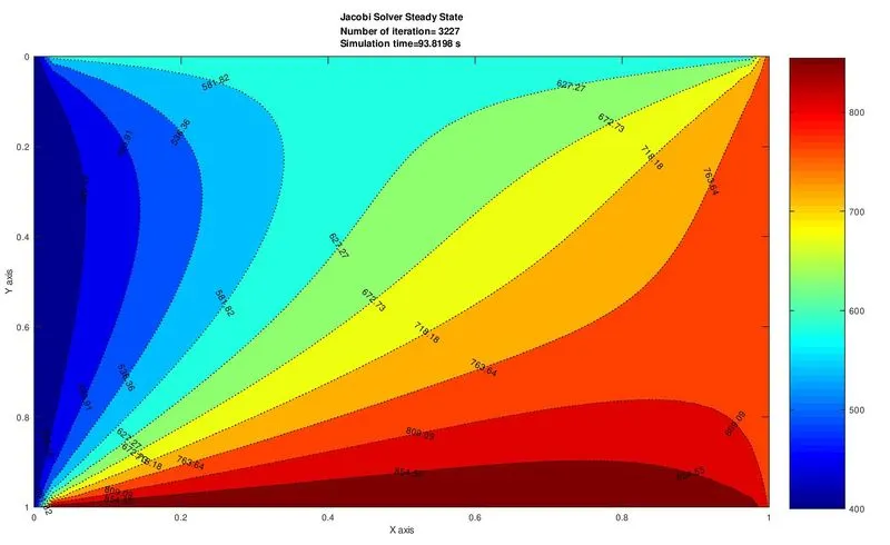
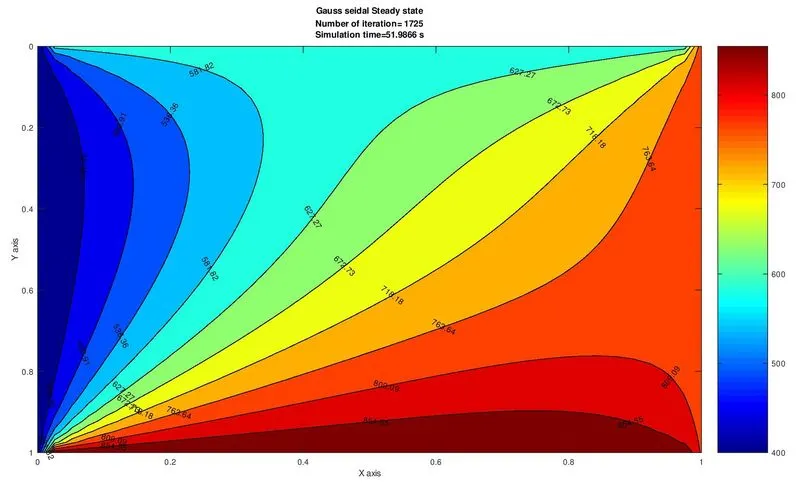
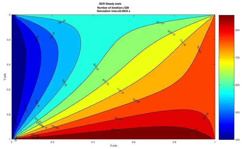
CONCLUSION :

We observe that the results are same in different methods, the different between them is number of iteration and computation time taken by iterative solver to get convergence result.
we can see that Jacobi iteration takes more number of iteration and computation time as compared to other two iterative solver this is because Jacobi iteration takes the old values.
While Gauss seidel and Successive over relaxiation(SOR) takes the updated values. Hence the new values is passed in new iteration as the solution proceeds.Thus in this type of iterative solver we get convergence result in less number of iteration as well as in less computation time.

SOLVING 2D HEAT CONDUCTION EQUATION FOR UNSTEADY STATE

Governing equation for 2D heat conduction equation for steady state

`(del^2T)/(delx^2)+(del^2T)/(dely^2)=0`

We've to solve the above governing equation by-

Explicit Scheme
Implicit Scheme

EXPLCIT SCHEME:

`((T^(n+1))_(i,j)-(T^n)_(i,j))/(Deltat)=alpha[((T^n)_(i+1,j)-(2T^n)_(i,j)+(T^n)_(i-1,j))/(Deltax^2)+((T^n)_(i,j+1)-(2T^n)_(i,j)+(T^n)_(i,j-1))/(Deltay^2)]^n`

`(T^(n+1))_(i,j)=(T^n)_(i,j)+alpha.Deltat[((T^n)_(i+1,j)-(2T^n)_(i,j)+(T^n)_(i-1,j))/(Deltax^2)+((T^n)_(i,j+1)-(2T^n)_(i,j)+(T^n)_(i,j-1))/(Deltay^2)]^n`

Let-

`(T^(n+1))_(i,j)=(T^(n+1))_(P)`

`(T^(n))_(i,j)=(T^(n))_(P)`

`(T^(n))_(i+1,j)=(T^(n))_(R)`

`(T^(n))_(i-1,j)=(T^(n))_(L)`

`(T^(n))_(i,j+1)=(T^(n))_(T)`

`(T^(n))_(i,j-1)=(T^(n))_(B)`

Therefore:

`(T^(n+1))_(P)=(T^n)_(P)+alpha.Deltat[((T^n)_(L)-(2T^n)_(P)+(T^n)_(R))/(Deltax^2)+((T^n)_(T)-(2T^n)_(P)+(T^n)_(B))/(Deltay^2)]^n`

`(T^(n+1))_(P)=(T^n)_(P)+k_1.(T_L-2T_P+T_R)^n+k_2.(T_T-2T_P+T_B)^n`

`(T^(n+1))_(P)=(T^n)_(P)(1-2k_1-2k_2)+k1.(T^n)_(L)+k1.(T^n)_(R)+k2.(T^n)_(T)+k2.(T^n)_(B)`

where - `k1=alpha(DeltaT)/(Deltax^2)` & `k2=alpha(DeltaT)/(Deltay^2)`

MAIN CODE 2:

%Solving transient 2D heat conduction equation EXPLICIT Method
clear all
close all
clc

%Input parameter
nx=40;  %no of grids-x-direction
ny=40;  %no of grids-y-direction
rf=1.5; %relaxation factor
dt=1e-4;
alpha=1.5;
nt=1400;

%Calculation
x=linspace(0,1,nx);
y=linspace(0,1,ny);
dx=x(2)-x(1); %Time step-x-direction
dy=y(2)-y(1); %Time step-y-direction

%Assigning BC
T=ones(nx,ny);
T(1,:)=600;   %Top Boundary
T(end,:)=900; %Bottom Boundary
T(:,1)=400;   %Left Boundary
T(:,end)=800; %Right Boundary
Told=T;

%Constant
k1=(alpha*dt)/(dx^2);
k2=(alpha*dt)/(dy^2);

tic
       for k=1:nt   %time loop
       for i=2:nx-1
       for j=2:ny-1
           Term1=(1-2*k1-2*k2);
           Term2=k1;
           Term3=k2;
           A=(Told(i-1,j)+Told(i+1,j));
           B=(Told(i,j-1)+Told(i,j+1));
           T(i,j)=(Told(i,j)*Term1)+(Term2*A)+(Term3*B);
       end
       end
            Told=T;
       end
           time1=toc;
           figure(1)
           colormap(jet)
           contourf(x,y,T,'showText','on')
           colorbar
           xlabel('x axis')
           ylabel('Y axis')
           set(gca,'YDIR','reverse');
           text2=sprintf('Simulation time=%d s',time1);
           title(['Transient State';text2]);
           colorbar
           pause(0.3)

RESULT 2:

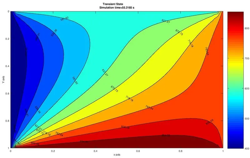
CONCLUSION :

In the transient solvers, the explicit schemes are usually easier to solve. This is because in the explicit case, we have a system of linear equations (nodes) that can be solved independently without iteration. This scheme actually works exactly like the steady case.
The time integration here is just the convergence loop in the steady case.The implicit solvers require iteration until convergence in the spatial node, plus then the same time integration as the explicit solvers. They are therefore computationally more expensive.

IMPLCIT SCHEME:

`((T^(n+1))_(i,j)-(T^n)_(i,j))/(Deltat)=alpha[((T^n)_(i+1,j)-(2T^n)_(i,j)+(T^n)_(i-1,j))/(Deltax^2)+((T^n)_(i,j+1)-(2T^n)_(i,j)+(T^n)_(i,j-1))/(Deltay^2)]^(n+1)`

`(T^(n+1))_(i,j)=(T^n)_(i,j)+alpha.Deltat[((T^n)_(i+1,j)-(2T^n)_(i,j)+(T^n)_(i-1,j))/(Deltax^2)+((T^n)_(i,j+1)-(2T^n)_(i,j)+(T^n)_(i,j-1))/(Deltay^2)]^(n+1)`

Let-

`(T^(n+1))_(i,j)=(T^(n+1))_(P)`

`(T^(n))_(i,j)=(T^(n))_(P)`

`(T^(n))_(i+1,j)=(T^(n))_(R)`

`(T^(n))_(i-1,j)=(T^(n))_(L)`

`(T^(n))_(i,j+1)=(T^(n))_(T)`

`(T^(n))_(i,j-1)=(T^(n))_(B)`

Therefore:

`((T^(n+1))_(P)-obrace((T^n)_(P))^(Known))/(Deltat)=alpha[ubrace[((T^n)_(L)-(2T^n)_(P)+(T^n)_(R))/(Deltax^2)+((T^n)_(T)-(2T^n)_(P)+(T^n)_(B))/(Deltay^2)]_("Unknown"")]^(n+1)`

So,

`(T^(n+1))_(P)=obrace((T^n)_(P))^(Known)+alpha.Deltat[ubrace[((T^n)_(L)-(2T^n)_(P)+(T^n)_(R))/(Deltax^2)+((T^n)_(T)-(2T^n)_(P)+(T^n)_(B))/(Deltay^2)]_("Unknown"")]^(n+1)`

`(T^(n+1))_(P)=(1)/(1+2.k_1+2.k_2)[(T^n)_(P)+k1(T_L+T_R)^(n+1)+k2(T_T+T_B)^(n+1)]`

where - `k1=alpha(DeltaT)/(Deltax^2)` & `k2=alpha(DeltaT)/(Deltay^2)`

so,

`Term_1=(1)/(1+2.k_1+2.k_2)`

`Term_2=k_1.(Term_1)`

`Term_3=k_1.(Term_2)`

Simplification : `(T^(n+1))_(P)=Term_1.(T^n)_(P)+Term_2.(T_L+T_R)^(n+1)+Term_3.(T_T+T_B)^(n+1)`

MAIN CODE 3:

%Solving the steady 2D heat conduction equation IMPLICIT Method
clear all
close all
clc

%Inputs
nx=40; %no of grids-x-direction
ny=40; %no of grids-y-direction
rf=1.5;%relexation factor
dt=1e-4;
alpha=1.5;
nt=1400;

%Calculation
x=linspace(0,1,nx);
y=linspace(0,1,ny);
dx=x(2)-x(1); %Time step-x-direction
dy=y(2)-y(1); %Time step-y-direction

%Assigning BC
T=ones(nx,ny);
T(1,:)=600;   %Top Boundary
T(end,:)=900; %Bottom Boundary
T(:,1)=400;   %Left Boundary
T(:,end)=800; %Right Boundary

Told=T;
Tprv=T;

%Constant
k1=(alpha*dt)/(dx^2);
k2=(alpha*dt)/(dy^2);

tol=1e-4; %tolerance

iterative_solver=input('enter iterative solver=')

%Jacobi Method
  jacobi_iter=1;
tic
if iterative_solver==1;
        for k=1:nt   %time loop
          error=9e9;  %error
           while (error>tol)
        for i=2:nx-1
        for j=2:ny-1
             Term1=(1+2*k1+2*k2)^-1;
             Term2=k1*Term1;
             Term3=k2*Term1;
             A=(T(i-1,j)+Told(i+1,j));
             B=(T(i,j-1)+Told(i,j+1));
             T(i,j)=(Term1*Tprv(i,j))+(Term2*A)+(Term3*B);
        end
      end
      error=max(max(abs(Told-T)));
      Told=T;
      jacobi_iter=jacobi_iter+1;
      end
      Tprv=T;
  end
  
     time1=toc;
     figure(1)
     colormap(jet)
     contourf(x,y,T,':','showText','on')
     xlabel('X axis')
     ylabel('Y axis')
     set(gca,'YDIR','reverse');
     text1=sprintf('Number of iteration= %d',jacobi_iter);
     text2=sprintf('Simulation time=%d s',time1);
     title(['Jacobi Solver Transient State';text1;text2]);
     colorbar
     pause(0.3)
end

%Gauss seidal Method
gs_iter=1;
tic 
if iterative_solver==2
   for k=1:nt   %time loop
          error=9e9;  %error
           while (error>tol)
        for i=2:nx-1
        for j=2:ny-1
             Term1=(1+2*k1+2*k2)^-1;
             Term2=k1*Term1;
             Term3=k2*Term1;
             A=(T(i-1,j)+Told(i+1,j));
             B=(T(i,j-1)+Told(i,j+1));
             T(i,j)=(Term1*Tprv(i,j))+(Term2*A)+(Term3*B);
        end
      end
      error=max(max(abs(Told-T)));
      Told=T;
      gs_iter=gs_iter+1;
      end
      Tprv=T;
   end

       time2=toc;
       figure(2)
       colormap(jet)
       contourf(x,y,T,'showText','on')
       xlabel('X axis')
       ylabel('Y axis')
       set(gca,'YDIR','reverse');
       text1=sprintf('Number of iteration= %d',gs_iter);
       text2=sprintf('Simulation time=%d s',time2);
       title(['Gauss seidal Transient state';text1;text2]);
       colorbar
       pause(0.03)
end

%SOR Method
sor_iter=1;
tic
if iterative_solver==3
   for k=1:nt   %time loop
          error=9e9;  %error
          while (error>tol)
            for i=2:nx-1
            for j=2:ny-1
                 Term1=(1+2*k1+2*k2)^-1;
                 Term2=k1*Term1;
                 Term3=k2*Term1;
                 A=(T(i-1,j)+Told(i+1,j));
                 B=(T(i,j-1)+Told(i,j+1));
                 T(i,j)=rf*((Term1*Tprv(i,j))+(Term2*A)+(Term3*B))+(1-rf)*Told(i,j);
            end 
            end
                  error=max(max(abs(Told-T)));
                  Told=T;
                  sor_iter=sor_iter+1;
          end
                 Tprv=T;
    end
          time3=toc;
           figure(3)
           colormap(jet)
           contourf(x,y,T,'showText','on')
           xlabel('X axis')
           ylabel('Y axis')
           set(gca,'YDIR','reverse');
           text1=sprintf('Number of iteration= %d',sor_iter);
           text2=sprintf('Simulation time=%d s',time3);
           title(['SOR Transient state';text1;text2]);
           colorbar
           pause(0.03)
end

RESULTS 3:

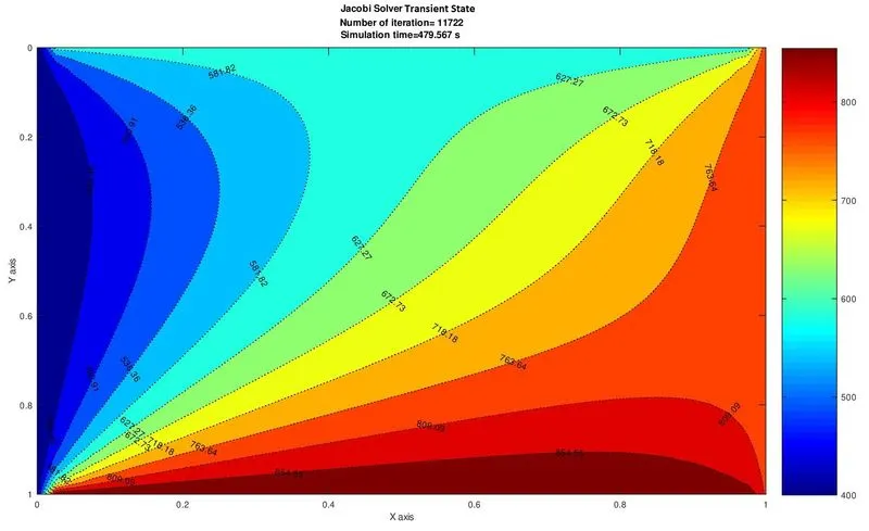
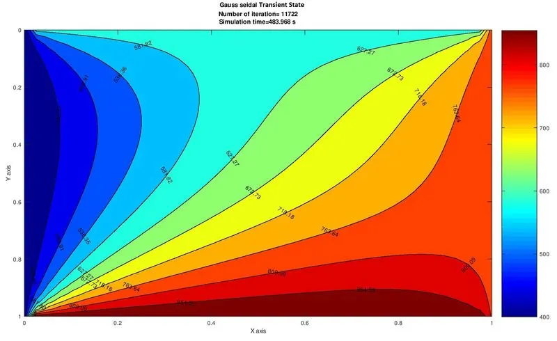
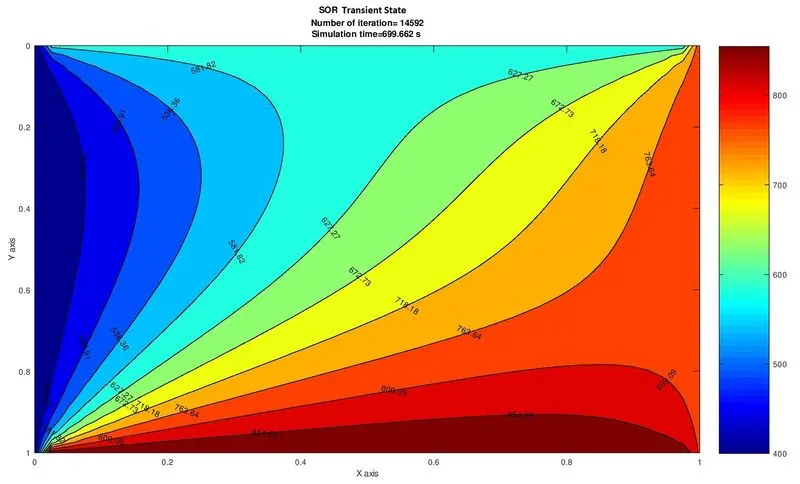
CONCLUSION :

We observe that the results are same in different methods, the different between them is number of iteration and computation time taken by iterative solver to get convergence result.
we can see that Jacobi iteration takes more number of iteration and computation time as compared to other two iterative solver this is because Jacobi iteration takes the old values.
Where as solver Gauss seidel & Successive over relaxiation (SOR) takes the updated values. Hence the new values is passed in new iteration as the solution proceeds.Thus in this type of iterative solver we get convergence result in less number of iteration as well as in less computation time.

Solving the steady and unsteady 2D heat conduction problem

Ship work like this
in your own course.

Talk to a career counsellor

Ship work like thisin your own course.

Talk to a career counsellor

Ship work like this
in your own course.