Week 5.1 - Mid term project - Solving the steady and unsteady 2D heat conduction problem
Jacobi Method for steay flow
clear all
close all
clc

%solving the steady state 2D equation (jacobi method)

%Input grids
nx=30;
ny=nx;

x=linspace(0,1,nx);
y= linspace(0,1,ny);

dx =x(2)-x(1);
dy= y(2)-y(1);

%error criteria
error= 9e9;
tol = 1e-4;

%defining the boundary condition
T_l= 400;
T_t= 600;
T_r= 800;
T_b= 900;

T= ones(nx,ny);

 T(2:ny-1,1) = T_l;
 T(2:ny-1,nx) = T_r;
 T(1,2:nx-1) = T_t;
 T(nx,2:ny-1) = T_b;

 %calculating the temperature at the corners
 T(1,1)=((T_t + T_l)/2);
 T(nx,ny) = ((T_r + T_b)/2);
 T(1,ny) = ((T_t + T_r)/2);
 T(nx,1) = ((T_l + T_b)/2);


 %assigning the T values
 T_intial = T;
 T_old = T;


  %jacobi method
  iterative_solver =1;

  if iterative_solver ==1
     jacobi_iter = 1;
     while (error > tol)
         for i = 2:nx-1
            for j = 2:ny-1
             T(i,j)=0.25*((T_old(i-1,j)+T_old(i+1,j)+T_old(i,j-1)+T_old(i,j+1)));
            end
         end

     error=max(max(abs(T_old-T)));
     T_old=T;
     jacobi_iter = jacobi_iter + 1;
     end


     % plotting
    figure(1)
    contourf(x,y,T)
    clabel(contourf(x,y,T))
    colorbar
    colormap(jet)

    xlabel('X_axis')
    ylabel('Y_axis')
    title_text=sprintf('Jacobi steady state No of iterations(implicit)=%d',jacobi_iter);
    title(title_text)
    pause(0.03);

  end
steady state Gauss Seidal method
clear all
close all
clc

%solving the steady state 2D equation (gs methid)

%Input grids
nx=30;
ny=nx;

x=linspace(0,1,nx);
y= linspace(0,1,ny);

dx =x(2)-x(1);
dy= dx;

%error criteria
error= 9e9;
tol = 1e-4;

%defining the boundary condition
T_l= 400;
T_r= 800;
T_t= 600;
T_b= 900;

T= 300*ones(nx,ny);

 T(2:ny-1,1) = T_l;
 T(2:ny-1,nx) = T_r;
 T(1,2:nx-1) = T_t;
 T(ny,2:nx-1) = T_b;

 %calculating the temperature at the corners
 T(1,1)=((T_t + T_l)/2);
 T(nx,ny) = ((T_r + T_b)/2);
 T(1,ny) = ((T_t + T_r)/2);
 T(nx,1) = ((T_l + T_b)/2);


 %assigning the T values
 T_intial = T;
 T_old = T;


  %gauss scidal method
  iterative_solver =2;
  if iterative_solver ==2
     gs_iter = 1;
     while (error > tol)
         for i = 2:nx-1
            for j = 2:ny-1
             T(i,j)=0.25*(T(i-1,j)+T_old(i+1,j)+T(i,j-1)+T_old(i,j+1));
            end
         end

     error=max(max(abs(T_old-T)));
     T_old=T;
     gs_iter = gs_iter + 1;
     end
     % plotting
    figure(1)
    contourf(x,y,T)
    clabel(contourf(x,y,T))
    colorbar
    colormap(jet)

    xlabel('X_axis')
    ylabel('Y_axis')
    title_text=sprintf('Gauss seidal steady state(implicit) No of iterations=%d',gs_iter);
    title(title_text)
    pause(0.03);

  end
Steady state with SOR method
clear all
close all
clc

%solving the steady state 2D equation (Sor methid)

%Input grids
nx=30;
ny=nx;

x=linspace(0,1,nx);
y= linspace(0,1,ny);

dx =x(2)-x(1);
dy= dx;

%error criteria
error= 9e9;
tol = 1e-4;
omega = 1.2;
%defining the boundary condition
T_l= 400;
T_r= 800;
T_t= 600;
T_b= 900;

T= 300*ones(nx,ny);

 T(2:ny-1,1) = T_l;
 T(2:ny-1,nx) = T_r;
 T(1,2:nx-1) = T_t;
 T(ny,2:nx-1) = T_b;

 %calculating the temperature at the corners
 T(1,1)=((T_t + T_l)/2);
 T(nx,ny) = ((T_r + T_b)/2);
 T(1,ny) = ((T_t + T_r)/2);
 T(nx,1) = ((T_l + T_b)/2);


 %assigning the T values
 T_intial = T;
 T_old = T;


  %gauss scidal method
  iterative_solver =3;
  if iterative_solver ==3
     sor_iter = 1;
     while (error > tol)
         for i = 2:nx-1
            for j = 2:ny-1
             T(i,j)=omega*(0.25*(T(i-1,j)+T_old(i+1,j)+T(i,j-1)+T_old(i,j+1)))+(1-omega)*T_old(i,j);
            end
         end

     error=max(max(abs(T_old-T)));
     T_old=T;
     sor_iter = sor_iter + 1;
     end
     % plotting
    figure(1)
    contourf(x,y,T)
    clabel(contourf(x,y,T))
    colorbar
    colormap(jet)

    xlabel('X_axis')
    ylabel('Y_axis')
    title_text=sprintf('SOR steady state (Implicit)No of iterations=%d',sor_iter);
    title(title_text)
    pause(0.03);

  end
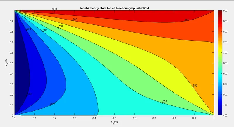
Jacobi steady state No of iterations(impilcit)
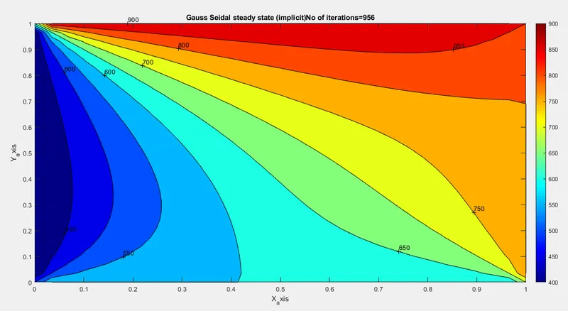
Gauss Seidal steady state (implicit)No of iterations
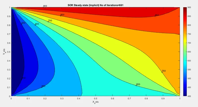
SOR Steady state (Implicit) No of iterations
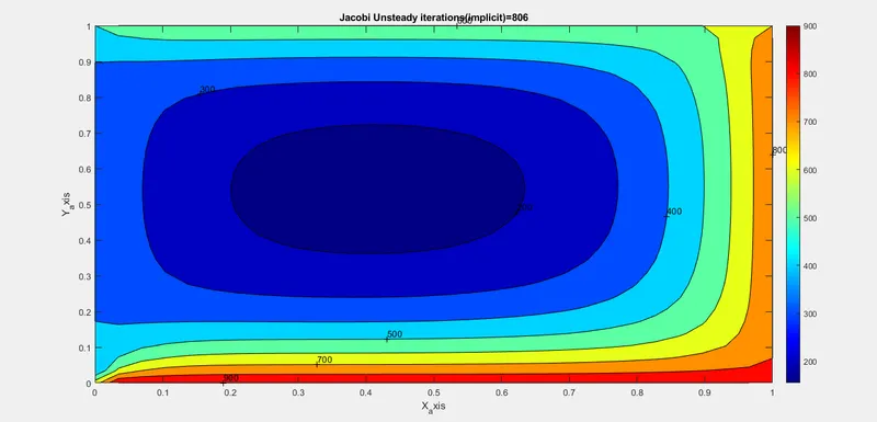
Transient state for Jacobi Method
clear all
close all
clc

%solving the  Unsteady state 2D equation (jacobi methid)

%Input grids
nx=30;
ny=nx;

x=linspace(0,1,nx);
y= linspace(1,0,ny);

dx =x(2)-x(1);
dy= y(2)-y(1);


%error criteria
error= 9e9;
tol = 1e-4;
dt=2000;
alpha=1.88e-5;

%defining the boundary condition
T_l= 400;
T_r= 800;
T_t= 600;
T_b= 900;

T= ones(nx,ny);

 T(2:ny-1,1) = T_l;
 T(2:ny-1,nx) = T_r;
 T(1,2:nx-1) = T_t;
 T(ny,2:nx-1) = T_b;

 %calculating the temperature at the corners
 T(1,1)=((T_t + T_l)/2);
 T(nx,ny) = ((T_r + T_b)/2);
 T(1,ny) = ((T_t + T_r)/2);
 T(nx,1) = ((T_l + T_b)/2);


 %assigning the T values
 T_intial = T;
 T_old = T;

 %calculating the 2D heat conduction equation by explicit
 k1=(alpha*dt)/(dx^2);
 k2=(alpha*dt)/(dy^2);
 T_prev_dt= T_old;

  %jacobi method
  term1= (1+2*k1+2*k2)^(-1);
  term2=k1*term1;
  term3=k2*term1;
  iterative_solver = 1;
  if iterative_solver ==1
      jacobi_iteration = 1;
     while (error > tol)
         for i = 2:nx-1
              for j = 2:ny-1
                H=(T_old(i-1,j)+T_old(i+1,j));
                V=(T_old(i,j-1)+T_old(i,j+1));
                T(i,j)=(T_prev_dt(i,j)*term1)+(H*term2+V*term3);
              end
         end

     error=max(max(abs(T_old-T)));
     T_old=T;
     jacobi_iteration = jacobi_iteration + 1;

    % plotting
    contourf(x,y,T)
    clabel(contourf(x,y,T))
    colorbar
    colormap(jet)
    xlabel('X_axis')
    ylabel('Y_axis')
    title_text=sprintf('Jacobi Unsteady iterations(implicit)=%d',jacobi_iteration);
    title(title_text)
    pause(0.03);
     end
  end
Transient State for Gauss Seidal
clear all
close all
clc

%solving the unsteady state 2D equation (gs method)

%Input grids
L=1;
nx=30;
ny=nx;

x=linspace(0,L,nx);
y= linspace(0,L,ny);

dx =x(2)-x(1);
dy= y(2)-y(1);


%error criteria
error= 9e9;
tol = 1e-4;
dt=2000;
alpha=1.88e-5;

%defining the boundary condition
T_l= 400;
T_t= 600;
T_r= 800;
T_b= 900;

T= ones(nx,ny);

 T(2:ny-1,1) = T_l;
 T(2:ny-1,nx) = T_r;
 T(1,2:nx-1) = T_t;
 T(ny,2:nx-1) = T_b;

 %calculating the temperature at the corners
 T(1,1)=((T_t + T_l)/2);
 T(nx,ny) = ((T_r + T_b)/2);
 T(1,ny) = ((T_t + T_r)/2);
 T(nx,1) = ((T_l + T_b)/2);


 %assigning the T values
 T_intial = T;
 T_old = T;

 %calculating the 2D heat conduction equation by explicit
 k1=(alpha*dt)/(dx^2);
 k2=(alpha*dt)/(dy^2);
 T_prev_dt= T_old;

  %gs method
  term1= (1+2*k1+2*k2)^(-1);
  term2=k1*term1;
  term3=k2*term1;
  iterative_solver = 2;
  if iterative_solver ==2
      gs_iteration = 1;
     while (error > tol)
         for i = 2:nx-1
              for j = 2:ny-1
                H=(T(i-1,j)+T_old(i+1,j));
                V=(T(i,j-1)+T_old(i,j+1));
                T(i,j)=(T_prev_dt(i,j)*term1)+(H*term2+V*term3);
              end
         end

     error=max(max(abs(T_old-T)));
     T_old=T;
     gs_iteration = gs_iteration + 1;

    % plotting
    contourf(x,y,T)
    clabel(contourf(x,y,T))
    colorbar
    colormap(jet)
    xlabel('X_axis')
    ylabel('Y_axis')
    title_text=sprintf('Gauss Seidal unsteady iterations(implicit)=%d',gs_iteration);
    title(title_text)
    pause(0.03);
     end
  end
Transient state For SOR Method
clear all
close all
clc

%solving the unsteady state 2D equation (SOR method)

%Input grids
L=1;
nx=30;
ny=nx;

x=linspace(0,L,nx);
y= linspace(0,L,ny);

dx =x(2)-x(1);
dy= y(2)-y(1);


%error criteria
error= 9e9;
tol = 1e-4;
dt=2000;
alpha=1.88e-5;

% For SOR
alpha1= 1.8;

%defining the boundary condition
T_l= 400;
T_t= 600;
T_r= 800;
T_b= 900;

T= ones(nx,ny);

 T(2:ny-1,1) = T_l;
 T(2:ny-1,nx) = T_r;
 T(1,2:nx-1) = T_t;
 T(ny,2:nx-1) = T_b;

 %calculating the temperature at the corners
 T(1,1)=((T_t + T_l)/2);
 T(nx,ny) = ((T_r + T_b)/2);
 T(1,ny) = ((T_t + T_r)/2);
 T(nx,1) = ((T_l + T_b)/2);


 %assigning the T values
 T_intial = T;
 T_old = T;

 %calculating the 2D heat conduction equation by explicit
 k1=(alpha*dt)/(dx^2);
 k2=(alpha*dt)/(dy^2);
 T_prev_dt= T_old;

  %SOR method
  term1= (1+2*k1+2*k2)^(-1);
  term2=k1*term1;
  term3=k2*term1;
  iterative_solver = 3;
  if iterative_solver == 3
      sor_iteration = 1;
     while (error > tol)
         for i = 2:nx-1
              for j = 2:ny-1
                H=(alpha1*T(i-1,j)+(1-alpha1)*T_old(i-1,j)+T_old(i+1,j));
                V=(alpha1*T(i,j-1)+(1-alpha1)*T_old(i,j-1)+T_old(i,j+1));
                T(i,j)=(T_prev_dt(i,j)*term1)+(H*term2+V*term3);
              end
         end

     error=max(max(abs(T_old-T)));
     T_old=T;
     sor_iteration = sor_iteration + 1;

    % plotting
    contourf(x,y,T)
    clabel(contourf(x,y,T))
    colorbar
    colormap(jet)
    xlabel('X_axis')
    ylabel('Y_axis')
    title_text=sprintf('Sor unsteady iterations(Implicit)=%d',sor_iteration);
    title(title_text)
    pause(0.03);
     end
  end
Transient (Implicit) for Jacobi Method
Transient Gauss Seidal
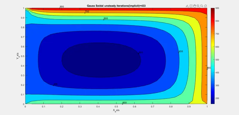
Transient SOR method
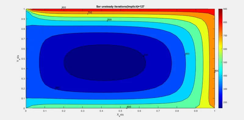
Transient Explicit
clear all
close all
clc

%solving the Transient state 2D equation for Explicit

%Input grids
nx=30;
ny=nx;
nt=1400;

x=linspace(0,1,nx);
y= linspace(0,1,ny);

dx =x(2)-x(1);
dy= y(2)-y(1);


%error criteria
error= 9e9;
tol = 1e-4;
dt=0.01;
alpha=1.88e-5;

%defining the boundary condition
T_l= 400;
T_r= 800;
T_t= 600;
T_b= 900;

T= ones(nx,ny);

 T(2:ny-1,1) = T_l;
 T(2:ny-1,nx) = T_r;
 T(1,2:nx-1) = T_t;
 T(nx,2:ny-1) = T_b;

 %calculating the temperature at the corners
 T(1,1)=((T_t + T_l)/2);
 T(nx,ny) = ((T_r + T_b)/2);
 T(1,ny) = ((T_t + T_r)/2);
 T(nx,1) = ((T_l + T_b)/2);


 %assigning the T values
 T_intial = T;
 T_old = T;

 %calculating the 2D heat conduction equation by explicit
 k1=(alpha*dt)/(dx^2);
 k2=(alpha*dt)/(dy^2);

    iterative_solver =1;
   if iterative_solver ==1
      explicit_iteration = 1;
     for k=1:nt
         error=1;
     while (error > tol)
         for i = 2:nx-1
              for j = 2:ny-1
                  term1= T_old(i,j);
                  term2= k1*(T_old(i+1,j)- 2*T_old(i,j)+(T_old(i-1,j)));
                  term3=k2*(T_old(i,j+1)- 2*T_old(i,j)+(T_old(i,j-1)));
                T(i,j)=(term1+term2+term3);
              end
         end
     error=max(max(abs(T_old-T)));
     T_old=T;
     explicit_iteration = explicit_iteration + 1;
     end
     end

    % plotting
    contourf(x,y,T)
    clabel(contourf(x,y,T))
    colorbar
    colormap(jet)
    xlabel('X_axis')
    ylabel('Y_axis')
    title_text=sprintf('Transient state for iterations(Explicit)=%d',explicit_iteration);
    title(title_text)
    pause(0.03);
   end
Transient Explicit 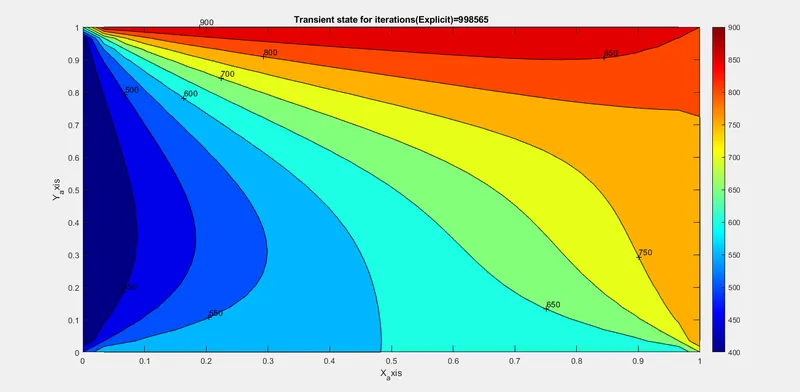
Table :
| Types | Methods | No. of iterations |
| Implicit- Steady |
Jacobi Gauss Seidal SOR |
1784 956 661 |
| Implicit- Unsteady |
Jacobi Gauss Seidal SOR |
806 433 127 |
| Explicit-Transient | 998565 |