Week 5.1 - Mid term project - Solving the steady and unsteady 2D heat conduction problem
Aim:
To solve steady as well as unsteady(transient) 2D heat conduction equation by using the point iterative techniques.
Theory:
The 2D heat conduction equation, eqn.1, is stated as follows,
`(delT)/(delt)+alpha((del^2T)/(delx^2)+(del^2T)/(dely^2))=0`
This equation can be solved by either steady state approach or transient state approach. For steady state, the time derivative term i.e. `(delT)/(delt)=0`. So, the equation, eqn.2, becomes,
`(del^2T)/(delx^2)+(del^2T)/(dely^2)=0`
For transient state, the time derivative and the space derivative terms remain. So, the eqn.1 is for transient state.
Solution of Steady state 2D heat conduction equation:
Eqn.2 can be solved by point iterative techniques i.e. Jacobi, Gauss-seidel, Successive over relaxation(SOR) method. But first, this PDE has to be converted into algebric equation. One can assign second order central difference scheme to space derivative term, such as the equation becomes,
`(T_(i-1,j)-2*T_(i,j)+T_(i+1,j))/(Deltax^2)+(T_(i,j-1)-2*T_(i,j)+T_(i,j+1))/(Deltay^2)=0`
After rearranging above equation we get, eqn.3,
`T_(i,j)=(Deltay^2)/(2*(Deltax^2+Deltay^2))(T_(i-1,j)+T_(i+1,j))+(Deltax^2)/(2*(Deltax^2+Deltay^2))(T_(i,j-1)+T_(i,j+1))`
where, `k1=(Deltay^2)/(2*(Deltax^2+Deltay^2))` and `k2=(Deltax^2)/(2*(Deltax^2+Deltay^2))`
For the sake of understanding, we can assume, `T_(i,j)=T_P`, `T_(i-1,j)=T_L`, `T_(i+1,j)=T_R`, `T_(i,j-1)=T_T`, `T_(i,j+1)=T_B`
So, the equation becomes, eqn.4,
`T_P=k1*(T_L+T_R)+k2*(T_T+T_B)`
This equation can be solved by using iterative methods i.e. Jacobi, Gauss-seidel, SOR method.
#Jacobi method
The eqn.4 changes to, eqn.5,
`T_P=k1*(T_(L(old))+T_(R(old)))+k2*(T_(T(old))+T_(B(old)))`
#Gauss-seidel method
The eqn.4 remains as it is.
#Successive Over Relaxation(SOR) method
The eqn.4 changes to, eqn.6,
`T_P=(1-omega)T_(P(old))+omega*(k1*(T_(L(old))+T_R)+k2*(T_(T(old))+T_B))`
Solution of Transient state 2D heat conduction equation:
For transient state, eqn.1 reamains as it is. Here, one can apply time marching scheme for time derivative and second order central differencing scheme for space derivative. Also, there are two types of equations i.e. explicit and implicit. In explicit equation, RHS values are known i.e values calculated at previous time step and so one can find LHS of the equation. On other hand, the implicit equation has unknowns on both sides i.e. both sides contain values of next time step.
In explicit type, eqn.1 changes to eqn.7,
`T_(i.j)^(n+1)=T_(i,j)^n-alpha*Deltat((T_(i+1,j)^n-2*T_(i,j)^n+T_(i-1,j)^n)/(Deltax^2)+(T_(i,j+1)^n-2*T_(i,j)^n+T_(i,j-1)^n)/(Deltay^2))`
In implicit type, eqn.1 changes to eqn.8,
`T_(i.j)^(n+1)=T_(i,j)^n-alpha*Deltat((T_(i+1,j)^(n+1)-2*T_(i,j)^(n+1)+T_(i-1,j)^(n+1))/(Deltax^2)+(T_(i,j+1)^(n+1)-2*T_(i,j)^(n+1)+T_(i,j-1)^(n+1))/(Deltay^2))`
By rearranging eqn.7 and using the nomenclature defined earlier, eqn.7 changes to eqn.9,
`T_P^(n+1)=1/(1+2k_1+2k_2)(T_p^n+k_1(T_L^n+T_R^n)+k_2(T_T^n+T_B^n))`
where, `k_1=(alpha*Deltat)/(Deltax^2)` and `k_2=(alpha*Deltat)/(Deltay^2)`
Similarly, eqn.8 changes to eqn.10,
`T_P^(n+1)=1/(1+2k_1+2k_2)(T_p^n+k_1(T_L^(n+1)+T_R^(n+1))+k_2(T_T^(n+1)+T_B^(n+1)))`
This equations can be solved by using iterative methods i.e. Jacobi, Gauss-seidel, SOR method.
#Jacobi method
Eqn.10 changes to eqn.11,
`T_P^(n+1)=1/(1+2k_1+2k_2)(T_p^n+k_1(T_(L(old))^(n+1)+T_R^(n+1))+k_2(T_(T(old))^(n+1)+T_B^(n+1)))`
#Gauss-seidel method
Eqn.10 reamains as it is.
#Successive Over Relaxation(SOR) method
Eqn.10 changes to eqn.12,
`T_P^(n+1)=(1-omega)*T_(P(old))^n+omega/(1+2k_1+2k_2)(T_p^n+k_1(T_L^(n+1)+T_R^(n+1))+k_2(T_T^(n+1)+T_B^(n+1)))`
Assumptions:
The Boundary conditions for the problem are as follows;
Top Boundary = 600 K
Bottom Boundary = 900 K
Left Boundary = 400 K
Right Boundary = 800 K
Tolerance = 1e-4
Starting error = 10
Domain length along x-axis and y-axis = 1m
Thermal diffusivity, `alpha`=1.4
Objectives:
- To solve the steady 2D heat conduction equation by using the point iterative techniques.
- To solve the unsteady 2D heat conduction equation by using the point iterative techniques.(for both explicit and implicit schemes)
MATLAB Program:
close all
clear all
clc

%Domain for evaluation
X=1;
Y=1;
nx=input('Enter number of nodes along x-axis: ');
ny=input('Enter number of nodes along y-axis: ');
dx=X/(nx-1);
dy=Y/(ny-1);
Here, domain length, number of nodes and distance between consecutive nodes, are defined.
%Initial values matrix
for k=1:nx
    for m=1:ny
        T(1,:)=600;
        T(:,1)=400;
        T(ny,:)=900;
        T(:,nx)=800;
    end
end
T(1,1)=500;
T(ny,1)=650;
T(ny,nx)=850;
T(1,nx)=700;

T_old=T;
T_pre_dt=T;
Here, initial values matrix is formed. All boundary conditions are set to the matrix. (1,:) assigns first row values for all columns. (:,1) assigns first column values for all rows. Similarly, other expressions are used to assign boundary conditions. After forming the matrix, it is saved under the names of 'T_old' and 'T_pre_dt'.
%Tolerance
tol=1e-4;
%Initial value of error between successive values of temperature
err_start=10;
%Thermal diffusivity
Alpha=1.4;
%Time step as per CFL
delta_T=0.5*((((dx^2)^-1)+((dy^2)^-1))^-1)/1.4;
%Relaxation factor
omega=1.4;
'delta_T' value is derived from CFL condition. The Courant–Friedrichs–Lewy or CFL condition is a condition for the stability of unstable numerical methods that model convection or wave phenomena. Therefore, the CFL condition expresses that the distance that any information travels during the timestep length within the mesh must be lower than the distance between mesh elements. In other words, information from a given cell or mesh element must propagate only to its immediate neighbors. For second order PDE, CFL condition is defined as follows,
`CFL_x+CFL_yle0.5`
where, `CFL_x=(alpha*Deltat)/(Deltax^2)`, `CFL_y=(alpha*Deltat)/(Deltay^2)`
Relaxation factor is useful in SOR method.
Solution of Steady state 2D heat conduction equation
equation=input('What type of equation 1.Steady or 2.Unsteady): ');
if equation==1
    fprintf('\nSteady 2D heat conduction equation\n\n')
%Iterative methods
fprintf('1. Jacobi method\n')
fprintf('2. Gauss-seidel method\n')
fprintf('3. Successive Over-lapping method\n')
'input' command takes values from user. Here, it is used for choosing between steady state and transient state solution. 'if-else' loop runs the functions of different iterative methods. 'fprintf' shows the text given in command.
%Steady 2d heat conduction
iterative_method=input('Enter number for iterative method to be used: ');

    if iterative_method==1
        T_jacobi=J_steady(err_start,tol,nx,ny,dx,dy,T,T_old)
    elseif iterative_method==2
        T_gs=GS_steady(err_start,tol,nx,ny,dx,dy,T,T_old)
    elseif iterative_method==3
        T_sor=SOR_steady(err_start,tol,nx,ny,dx,dy,T,T_old,omega)
    end
After selecting '1' from first input command, the program shows the options for steady state equation's solution. The options include, 'J_steady', 'GS_steady', 'SOR_steady'. These functions are explained below.
#Function for Jacobi method
function T_jacobi=J_steady(err_start,tol,nx,ny,dx,dy,T,T_old)
%Steady 2d heat conduction
itr=1;
 while err_start > tol %Convergence loop
 for i=2:nx-1 %Space loop
    for j=2:ny-1
        k1=0.5*(dy^2)/(dx^2+dy^2);
        k2=0.5*(dx^2)/(dx^2+dy^2);
        term1=k1*(T_old(i-1,j)+T_old(i+1,j));
        term2=k2*(T_old(i,j-1)+T_old(i,j+1));
        T(i,j)=term1+term2;
    end
 end
 err_start=max(max(abs(T_old-T)));
 T_old=T;
 itr=itr+1;
 end
 T_jacobi=T;
 fprintf('Error is %d\n',err_start)
 fprintf('No. of iterations required: %d',itr)
 T=flip(T);
contourf(T,'showtext','on')
colormap(parula)
colorbar
xlabel('X-axis')
ylabel('Y-axis')
title('Solution of Steady 2D heat conduction equation by using Jacobi method')
end
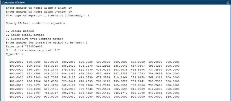
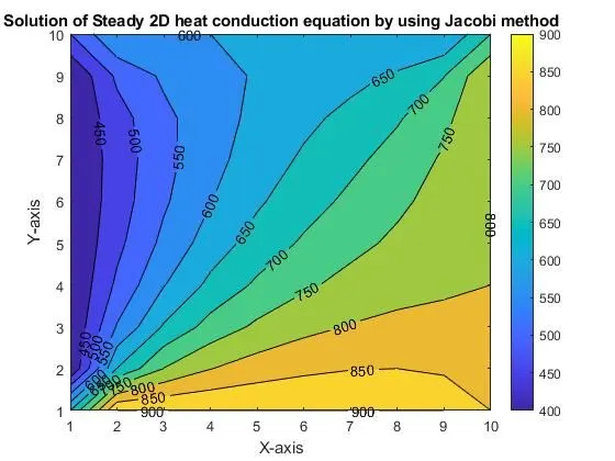
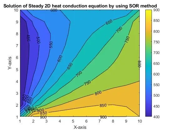
'itr' saves number of iterations required for converging the solution. For that convergence loop is used, which is a 'for' loop. The terms starting error and tolerance defined earlier will be useful here. 'err_start' is the starting error and 'tol' is the tolerance. For solution to get converged, the 'err_start' should be less that 'tol'. Inside convergence loop, there is a space loop. This loop calculates tempearture values at each node excluding boundary nodes. The formula defined earlier for Jacobi method, is used here (eqn.5). After space loop, 'err_start' is calculated. If it is below 'tol' then loop ends otherwise it continues. Also, 'T_old' get updated after each iteration in space loop. After convergence loop, T values are saved in 'T_jacobi'. To plot the results, 'contourf' command is used. Before that the values are flipped so they represent the order of nodes in matrix 'T'. 'colormap' type 'parula' is chosen. Labels and title are given.
#Function for Gauss-seidel method
function T_gs=GS_steady(err_start,tol,nx,ny,dx,dy,T,T_old)
%Steady 2d heat conduction
itr=1;
 while err_start > tol
 for i=2:nx-1
    for j=2:ny-1
        k1=0.5*(dy^2)/(dx^2+dy^2);
        k2=0.5*(dx^2)/(dx^2+dy^2);
        term1=k1*(T(i-1,j)+T_old(i+1,j));
        term2=k2*(T(i,j-1)+T_old(i,j+1));
        T(i,j)=term1+term2;
    end
 end
 err_start=max(max(abs(T_old-T)));
 T_old=T;
 itr=itr+1;
 end
 T_gs=T;
 fprintf('Error is %d\n',err_start)
 fprintf('No. of iterations required: %d',itr)
 T=flip(T);
contourf(T,'showtext','on')
colormap(parula)
colorbar
xlabel('X-axis')
ylabel('Y-axis')
title('Solution of Steady 2D heat conduction equation by using Gauss-seidel method')
end
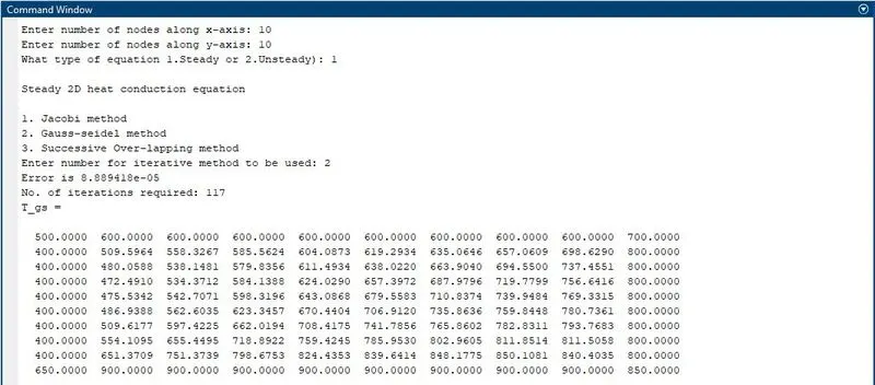
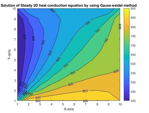
All things remain same except the formula used for calculating T(i,j). Refer 'Theory' section for explanation (eqn.4).
#Function for SOR method
function T_sor=SOR_steady(err_start,tol,nx,ny,dx,dy,T,T_old,omega)
%Steady 2d heat conduction
itr=1;
 while err_start > tol
 for i=2:nx-1
    for j=2:ny-1
        k1=0.5*(dy^2)/(dx^2+dy^2);
        k2=0.5*(dx^2)/(dx^2+dy^2);
        term1=k1*(T(i-1,j)+T_old(i+1,j));
        term2=k2*(T(i,j-1)+T_old(i,j+1));
        T(i,j)=(1-omega)*T_old(i,j)+omega*(term1+term2);
    end
 end
 err_start=max(max(abs(T_old-T)));
 T_old=T;
 itr=itr+1;
 end
 T_sor=T;
 fprintf('Error is %d\n',err_start)
 fprintf('No. of iterations required: %d',itr)
 T=flip(T);
contourf(T,'showtext','on')
colormap(parula)
colorbar
xlabel('X-axis')
ylabel('Y-axis')
title('Solution of Steady 2D heat conduction equation by using SOR method')
end
All things remain same except the formula used for calculating T(i,j). Refer 'Theory' section for explanation (eqn.6).
Solution of Transient state 2D heat conduction equation
%Unsteady 2d heat conduction
elseif equation==2
    method=input('1. Explicit or 2. Implicit: ');
    %Explicit
    if method==1
        fprintf('\nUnsteady 2D heat conduction equation\n\n')
        T_trans_explicit= unsteady_2d_heat_conduction_explicit(tol,nx,ny,Alpha,delta_T,dx,dy,T,T_old)
Transient state equation can be solved by two approaches i.e. explicit and implicit. Here, 'input' command takes input from user regarding 'Explicit' and 'Implicit'. The function 'unsteady_2d_heat_conduction_explicit' is used to solve the equation by explicit approach.
#Function for explicit approach
function T_trans_explicit= unsteady_2d_heat_conduction_explicit(tol,nx,ny,Alpha,delta_T,dx,dy,T,T_old)
itr=1;
for k=1:1400
    err_start=10;
    while err_start>tol
    for i=2:nx-1
        for j=2:ny-1
            k1=(Alpha*delta_T)/(dx^2);
            k2=(Alpha*delta_T)/(dy^2);
            term1=k1*(T_old(i-1,j)+T_old(i+1,j));
            term2=k2*(T_old(i,j-1)+T_old(i,j+1));
            T(i,j)=((1+2*k1+2*k2)^-1)*(T_old(i,j)+term1+term2);
        end
    end
    err_start=max(max(abs(T_old-T)));
    T_old=T;
    itr=itr+1;
    end
end
T_trans_explicit=T;
fprintf('Error is %d\n',err_start)
fprintf('No. of iterations required: %d',itr)
T=flip(T);
contourf(T,'showtext','on')
colormap(parula)
colorbar
xlabel('X-axis')
ylabel('Y-axis')
title('Solution of Unsteady 2D heat conduction equation(explicit)')
end
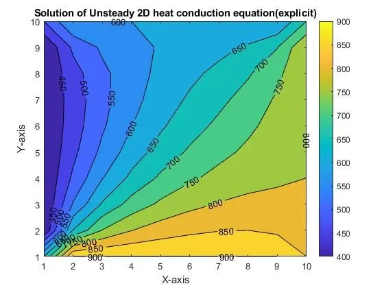
Here, alongwith convergence and space loops, time loop is used. 'err_start' has to be defined before convergence loop. So, everytime convergence loop ends, the initial error value will get used for the loop. Also, k1 and k2 values are changed. Refer 'Theory' section for explanation (eqn.9).
%Implicit
    elseif method==2
        fprintf('\nUnsteady 2D heat conduction equation\n\n')
        %Iterative methods
        fprintf('1. Jacobi method\n')
        fprintf('2. Gauss-seidel method\n')
        fprintf('3. Successive Over-lapping method\n')

        iterative_method_trans=input('Enter number for iterative method to be used: ');
            if iterative_method_trans==1
                T_trans_j=J_unsteady(err_start,tol,nx,ny,dx,dy,Alpha,delta_T,T,T_old,T_pre_dt)
            elseif iterative_method_trans==2
                T_trans_gs=GS_unsteady(err_start,tol,nx,ny,dx,dy,Alpha,delta_T,T,T_old,T_pre_dt)
            elseif iterative_method_trans==3
                T_trans_sor=SOR_unsteady(err_start,tol,nx,ny,dx,dy,Alpha,delta_T,T,T_old,T_pre_dt,omega)
            end
    end
end
'input' command allows user to choose implicit approach as well. These contains again three functions for three iterative methods.
#Function for Jacobi method
function T_trans_j=J_unsteady(err_start,tol,nx,ny,dx,dy,Alpha,delta_T,T,T_old,T_pre_dt)
itr=1;
for p=1:1400
    err_start=10;
    while err_start>tol
    for i=2:nx-1
        for j=2:ny-1
            k1=(Alpha*delta_T)/(dx^2);
            k2=(Alpha*delta_T)/(dy^2);
            term1=k1*(T_old(i-1,j)+T_old(i+1,j));
            term2=k2*(T_old(i,j-1)+T_old(i,j+1));
            T(i,j)=((1+2*k1+2*k2)^-1)*(T_pre_dt(i,j)+term1+term2);
        end
    end
    err_start=max(max(abs(T_old-T)));
    T_old=T;
    itr=itr+1;
    end
    T_pre_dt=T;
end
T_trans_j=T;
fprintf('Error is %d\n',err_start)
fprintf('No. of iterations required: %d',itr)
T=flip(T);
contourf(T,'showtext','on')
colormap(parula)
colorbar
xlabel('X-axis')
ylabel('Y-axis')
title('Solution of Unsteady 2D heat conduction equation(implicit) by using Jacobi method')
end
Here, the only change is the value of 'T_pre_dt'. This matrix is for previous time step T values. Refer 'Theory' section for explanation (eqn.11). This 'T_pre_dt' gets updated after each convergence loop's iteration. Apart from this, the logic is same as that for explicit approach.
#Function for Gauss-seidel method
function T_trans_gs=GS_unsteady(err_start,tol,nx,ny,dx,dy,Alpha,delta_T,T,T_old,T_pre_dt)
itr=1;
for p=1:1400
    err_start=10;
    while err_start>tol
    for i=2:nx-1
        for j=2:ny-1
            k1=(Alpha*delta_T)/(dx^2);
            k2=(Alpha*delta_T)/(dy^2);
            term1=k1*(T(i-1,j)+T_old(i+1,j));
            term2=k2*(T(i,j-1)+T_old(i,j+1));
            T(i,j)=((1+2*k1+2*k2)^-1)*(T_pre_dt(i,j)+term1+term2);
        end
    end
    err_start=max(max(abs(T_old-T)));
    T_old=T;
    itr=itr+1;
    end
    T_pre_dt=T;
end
T_trans_gs=T;
fprintf('Error is %d\n',err_start)
fprintf('No. of iterations required: %d',itr)
T=flip(T);
contourf(T,'showtext','on')
colormap(parula)
colorbar
xlabel('X-axis')
ylabel('Y-axis')
title('Solution of Unsteady 2D heat conduction equation(implicit) by using Gauss-seidel method')
end
All things remain same except the formula used for calculating T(i,j). Refer 'Theory' section for explanation (eqn.10).
#Function for SOR method
function T_trans_sor=SOR_unsteady(err_start,tol,nx,ny,dx,dy,Alpha,delta_T,T,T_old,T_pre_dt,omega)
itr=1;
for p=1:1400
    err_start=10;
    while err_start>tol
    for i=2:nx-1
        for j=2:ny-1
            k1=(Alpha*delta_T)/(dx^2);
            k2=(Alpha*delta_T)/(dy^2);
            term1=((1+2*k1+2*k2)^-1);
            term2=k1*(T(i-1,j)+T_old(i+1,j));
            term3=k2*(T(i,j-1)+T_old(i,j+1));
            T(i,j)=(1-omega)*T_old(i,j)+omega*(term1*(T_pre_dt(i,j)+term2+term3));
        end
    end
    err_start=max(max(abs(T_old-T)));
    T_old=T;
    itr=itr+1;
    end
    T_pre_dt=T;
end
T_trans_sor=T;
fprintf('Error is %d\n',err_start)
fprintf('No. of iterations required: %d',itr)
T=flip(T);
contourf(T,'showtext','on')
colormap(parula)
colorbar
xlabel('X-axis')
ylabel('Y-axis')
title('Solution of Unsteady 2D heat conduction equation(implicit) by using SOR method')
end
All things remain same except the formula used for calculating T(i,j). Refer 'Theory' section for explanation (eqn.12).
Outputs:
Solution of steady state 2D heat conduction equation using Jacobi method
#1
#2
Solution of steady state 2D heat conduction equation using Gauss-seidel method
#1
#2
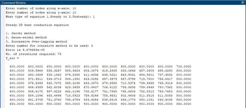
Solution of steady state 2D heat conduction equation using SOR method
#1
#2
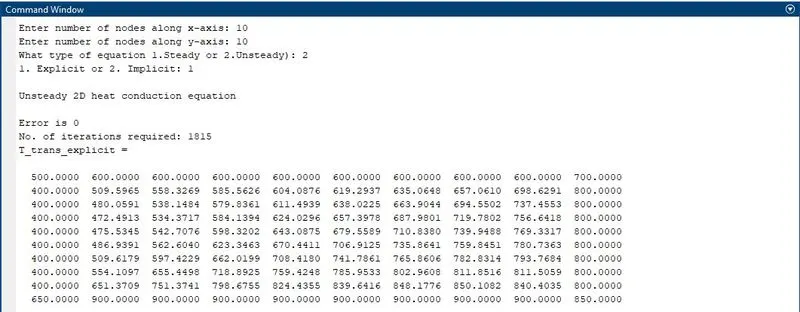
Solution of unsteady state 2D heat conduction equation using explicit method
#1
#2
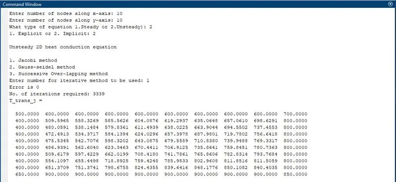
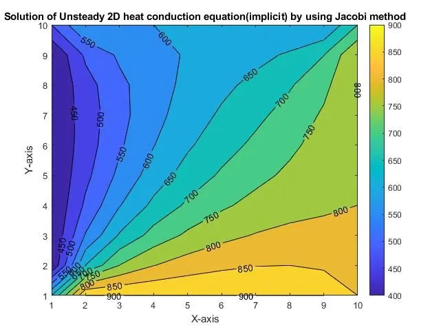
Solution of unsteady state 2D heat conduction equation using Jacobi method
#1
#2
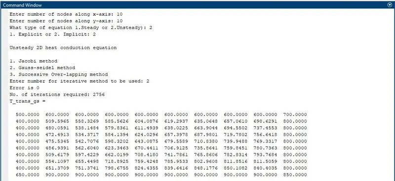
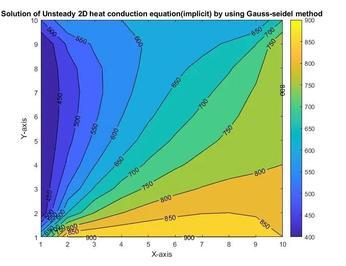
Solution of unsteady state 2D heat conduction equation using Gauss-seidel method
#1
#2
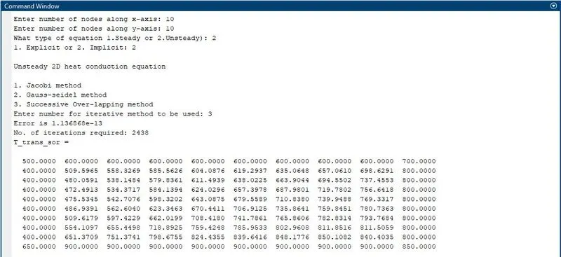
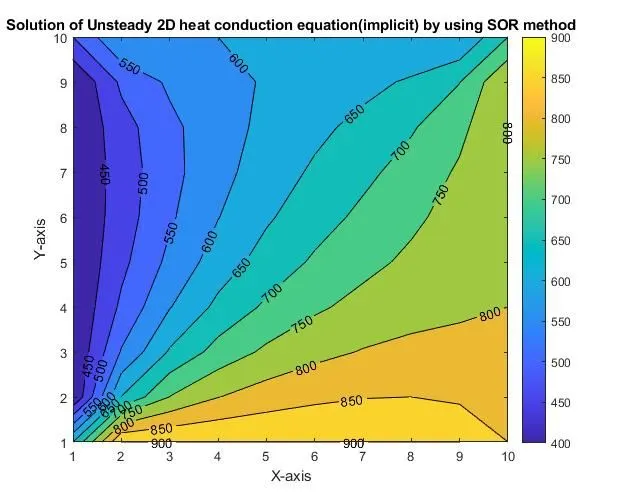
Solution of unsteady state 2D heat conduction equation using SOR method
#1
#2
Conlusion:
- It is observed that the iteration required for convergence decreases with an order of iterative methods i.e. Jacobi method, Gauss-seidel method, SOR method.
- Transient state equation requires more number of iterations to solve than the steady state equation.
- Increase in the Relaxation factor used in SOR method, helps to reach solution faster upto certain value of `omega`.